Data presentation: histograms, box plots, measures and outliers Statistics
Papers
Paper 2, Paper 2 (Statistics), Paper 3, Paper 3 (Statistics)
Level
AS and A level
Spec
S2.1, S2.3, S2.4
Booklet
The standard deviation formula is given.
Since 2018
73 question parts, 146 marks, 7 with a difficulty rating from the examiner's report
Notes, worked examples and practice for this topic are being written by our tutors. The past-paper questions below are ready now: work each one on paper, then open the mark scheme and the examiner's comment.
Tap a question to zoom it. Mark scheme and examiner's comment open under each question.
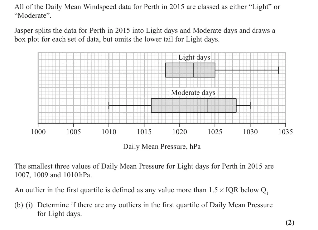
June 2025 · AS Paper 2 (Statistics) · Q2(b)(i)2 marks
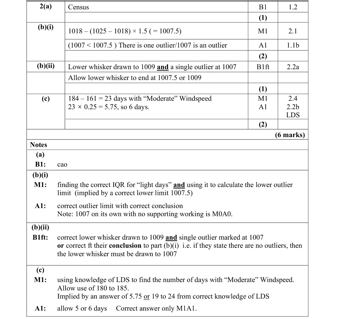
Mark scheme (whole question; this part is marked with the orange bar)
Examiner's comment
Most students were able to complete part (b)(i), calculating the lower outlier limit correctly and then showing that 1007 was an outlier. The most common mistakes were calculating 1007.5 but then concluding there were no outliers or only finding the IQR and thus attaining no marks. The drawing of outliers on a boxplot caused problems, with many students getting (b)(i) correct but then being unable to illustrate this correctly on the box plot. Often students made bottom whisker end at 1009 but did not mark in the outlier. There was also a significant minority who were unable to read the scale correctly when plotting values. There was follow through available in (b)(ii) for those who made a slip calculating the lower outlier limit in
Common mistakes
read Q1 = 1018 and Q3 = 1025 from the box plot
limit 1018 − 1.5 × 7 = 1007.5
conclude 1007 is the only outlier (1007 alone with no working scores 0)
some found 1007.5 then said there were no outliers, or found only the IQR
June 2025 · AS Paper 2 (Statistics) · Q2(b)(ii)1 mark
Mark scheme (whole question; this part is marked with the orange bar)
Examiner's comment
through available in (b)(ii) for those who made a slip calculating the lower outlier limit in part (i).
Common mistakes
lower whisker to 1009 (1007.5 allowed) and a single outlier marked at 1007
many drew the whisker but did not mark the outlier, or misread the scale
June 2025 · AS Paper 2 (Statistics) · Q2(c)2 marks
Mark scheme (whole question; this part is marked with the orange bar)
Examiner's comment
Part (c) proved more challenging for most, demonstrating that students are still not familiar with the large data set and how to apply it to a scenario. Of the students who were able to successfully identify the number of moderate days, most were able to make use of the upper quartile to arrive at a correct estimate of 5 or 6 days. A small number of students calculated three quarters of the days instead of one quarter.
Common mistakes
needs LDS knowledge that Perth 2015 has 184 days (May to October) so 184 − 161 = 23 Moderate days
1028 is the upper quartile for Moderate days so a quarter: 23 × 0.25 = 5.75, so 5 or 6 days
some used three quarters
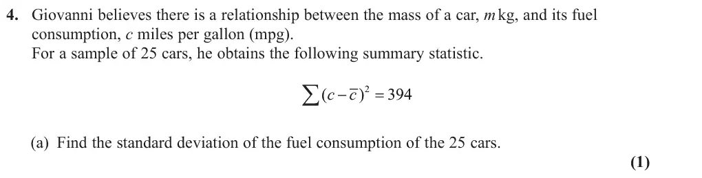
June 2025 · AS Paper 2 (Statistics) · Q4(a)1 mark
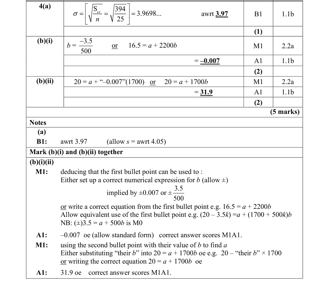
Mark scheme (whole question; this part is marked with the orange bar)
Examiner's comment
In part (a), it appeared that many students did not recognise the sum given as that used in the Common errors were sqrt 394 and 394 original definition of variance/standard deviation and so were unable to attempt an answer. 25 although other wrong solutions involving extensive calculations were also seen. For part (b) many students misinterpreted the information in the first bullet point and used the
Common mistakes
recognise Σ(c − c̄)² = Scc so sd = √(394/25) = 3.97 (s = 4.05 allowed)
common errors √394 and 394/25
June 2025 · Paper 3 (Statistics) · Q2(a)1 mark
Mark scheme (whole question; this part is marked with the orange bar)
Examiner's comment
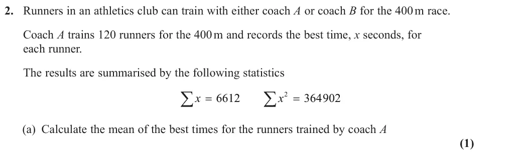
The majority of learners answered parts (a) and (b) very well. A very small minority used 364902 6612 in part (a) and a sizeable number found the variance not the standard deviation in
Common mistakes
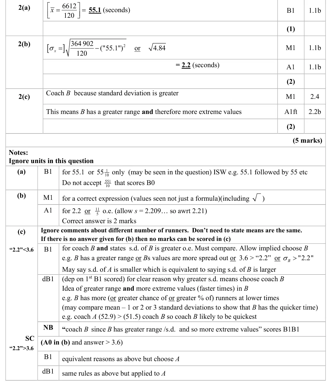
mean = 6612/120 = 55.1
June 2025 · Paper 3 (Statistics) · Q2(b)2 marks
Mark scheme (whole question; this part is marked with the orange bar)
Examiner's comment
The majority of learners answered parts (a) and (b) very well. A very small minority used 364902 6612 in part (a) and a sizeable number found the variance not the standard deviation in part (b).
Common mistakes
σ = √(364902/120 − 55.1²) = 2.2
giving the variance 4.84 instead of the standard deviation
June 2025 · Paper 3 (Statistics) · Q2(c)2 marks
Mark scheme (whole question; this part is marked with the orange bar)
Examiner's comment
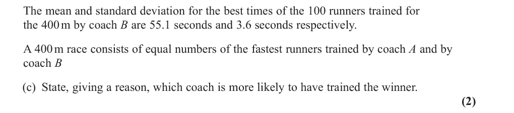
Part (c) proved to be more challenging with many choosing coach A on the basis that the lower standard deviation meant that those runners would be more “consistent”. A good number of responses chose coach B citing the larger standard deviation as a reason, but few were able to explain that the larger standard deviation increases the likelihood of an extreme value such as the fastest time. A small minority of responses did not consider standard deviation and instead incorrectly focused on the different sample sizes.
Common mistakes
same mean, so coach B because the larger standard deviation means more extreme (faster) times
"A is more consistent" is wrong
sample sizes are irrelevant
June 2025 · Paper 3 (Statistics) · Q4(b)1 mark
Mark scheme (whole question; this part is marked with the orange bar)
Examiner's comment
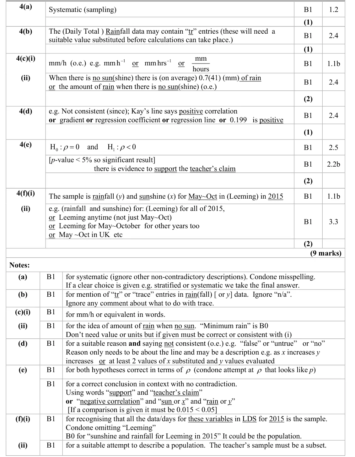
In part (b) most identified that “trace” or “tr” would need attention, but some did not link this to the rainfall variable. In part (c) (i) there were many correct answers and some who
Common mistakes
daily total rainfall may contain "tr" (trace) entries that need a value before calculating
must link it to rainfall
June 2024 · AS Paper 2 (Statistics) · Q14 marks
Mark scheme (whole question; this part is marked with the orange bar)
Examiner's comment
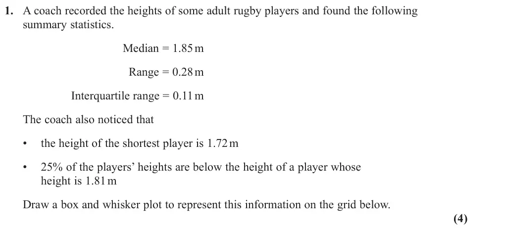
This question proved to be a successful start to the paper for most students, with many scoring full marks. Those who struggled did not recognise that 25% of the players' heights represented the lower quartile. They were still able to draw the interquartile range to the correct distance. Most students were able to correctly draw the whiskers for the lower and upper values, but there were a small minority who have no idea what a box and whisker diagram should look like, and some just plotted points or simply vertical drew lines.
Common mistakes
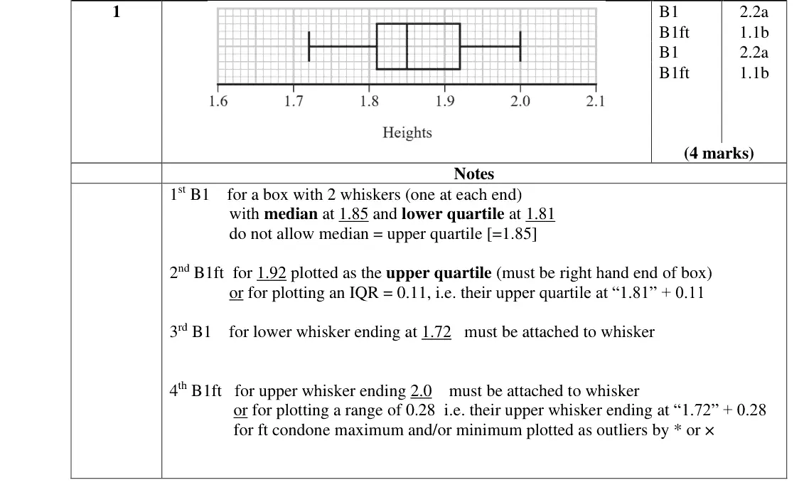
"25% below 1.81" means Q1 = 1.81
Q3 = 1.81 + 0.11 = 1.92
whiskers from 1.72 to 1.72 + 0.28 = 2.00
median 1.85 inside the box (not equal to Q3)
some plotted points or vertical lines only
June 2024 · AS Paper 2 (Statistics) · Q2(a)1 mark
Mark scheme (whole question; this part is marked with the orange bar)
Examiner's comment
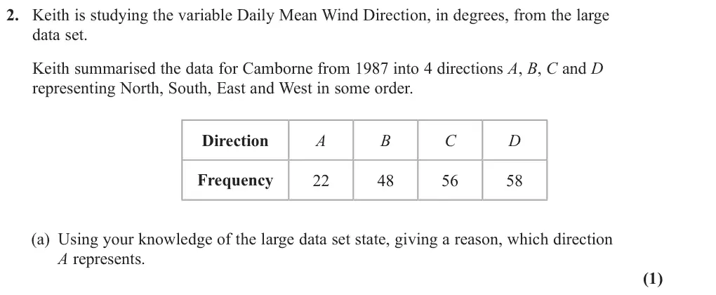
This question was generally not well attempted demonstrating that students are still not completely familiar with the large data set. In part (a) many students appeared to be aware of Camborne's location in the South-West of the UK but could not relate this to the prevailing winds in that area. Some students were able to guess that A represented East but were unable to provide a reason. Many students did not appreciate that wind direction is the direction that wind blows from, rather than to.
Common mistakes
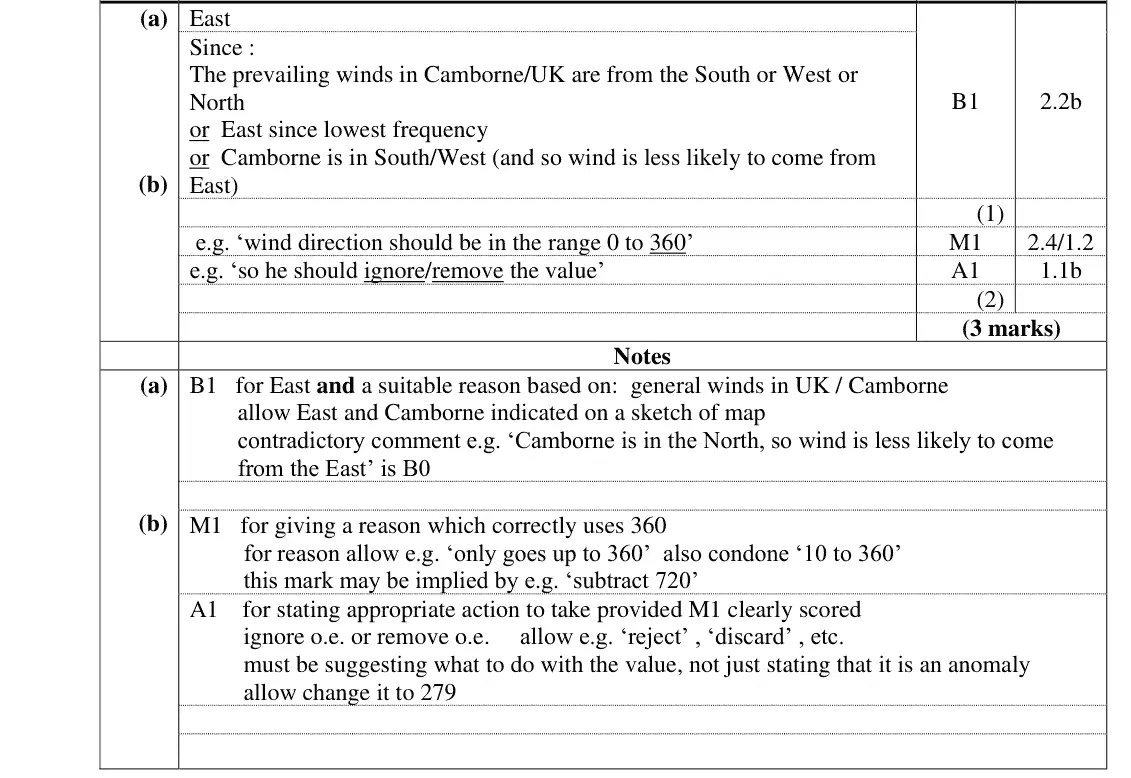
A is East: the least common direction, since prevailing UK/Camborne winds come from the south-west (west/south)
wind direction is where the wind blows from, not to
a reason is needed
June 2024 · AS Paper 2 (Statistics) · Q2(b)2 marks
Mark scheme (whole question; this part is marked with the orange bar)
Examiner's comment
This question was generally not well attempted demonstrating that students are still not In part (b), many students appreciated that the value was an outlier and should be excluded but were unable to score the marks here without justification. Those who understood that the maximum that the angle could be 360, tended to score well here. Some students also thought that 999 represented a frequency rather than an angle.
Common mistakes
wind direction runs from 0 to 360 degrees so 999 is not a valid value (it is an error/missing-data code, not an outlier or a frequency)
remove/ignore it
a reason using 360 is needed before the action
June 2024 · AS Paper 2 (Statistics) · Q3(a)2 marks
Mark scheme (whole question; this part is marked with the orange bar)
Examiner's comment
Part (a) was well attempted and almost all students realised that the two missing frequencies should sum to 32.
Common mistakes
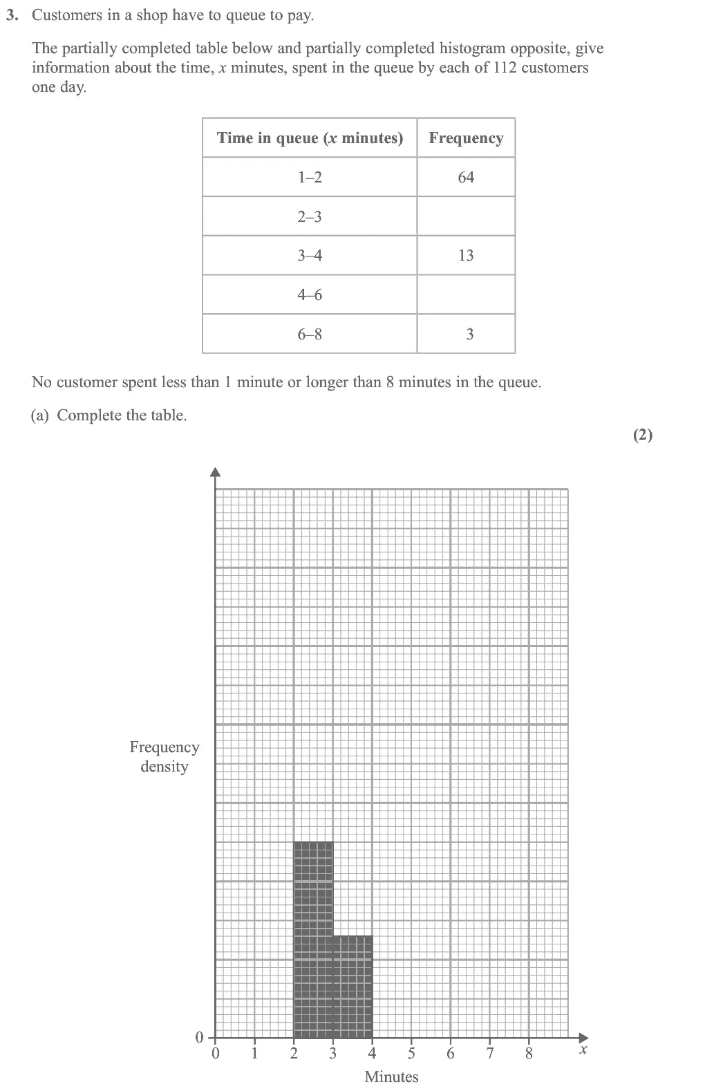
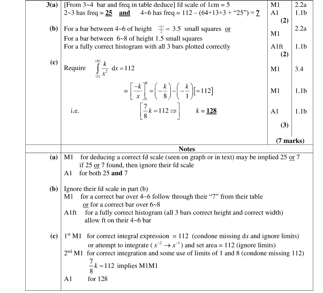
deduce the frequency density scale from the 3–4 bar (frequency 13)
2–3 has frequency 25 and 4–6 has 112 − (64 + 25 + 13 + 3) = 7
the two missing frequencies sum to 32
June 2024 · AS Paper 2 (Statistics) · Q3(b)2 marks
Mark scheme (whole question; this part is marked with the orange bar)
Examiner's comment
In part (b), the most usual mistake was to use frequency rather than frequency density for the heights of the 4 – 6 and 6 – 8 bars, drawing them at 7 small squares and 3 small squares respectively. Also, the first bar was often seen drawn from 0 – 2 instead of 1 – 2 often with an incorrect height.
Common mistakes
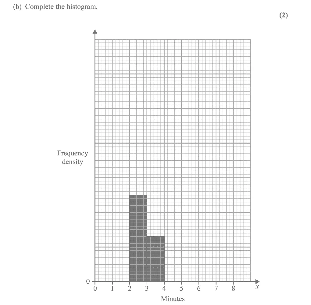
bar heights are frequency densities: 4–6 bar height 7/2 = 3.5 and 6–8 bar height 1.5
drawing heights as frequencies (7 and 3)
first bar must run from 1 to 2, not 0 to 2
June 2024 · AS Paper 2 (Statistics) · Q3(c)3 marks
Mark scheme (whole question; this part is marked with the orange bar)
Examiner's comment
Part (c) was not well done and quite often no attempt was made. Some students substituted one or more values of x, setting the result equal to the frequency (or frequency density). When integration was used, it was often done well. It was, however, surprising to see that even when the correct integration was equated to 112, many were unable to accurately solve the equation. Many students made slips with the negative signs, and some were unable to solve the equation, multiplying one side by 8 to get rid of the fraction but failing to multiply 112 by 8 at the same time.
Common mistakes
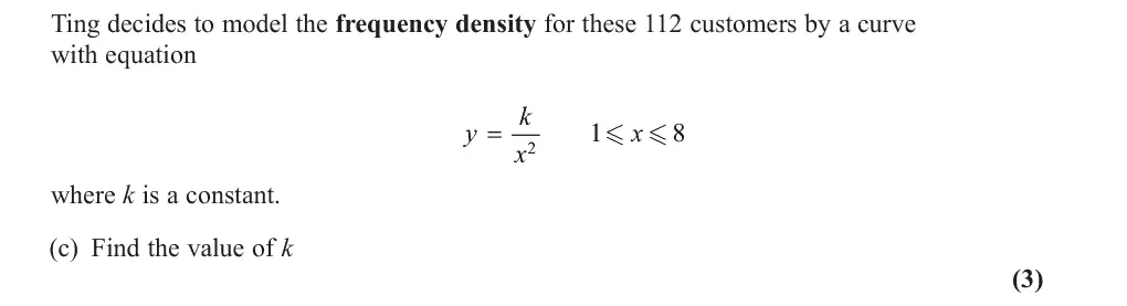
area under the frequency density curve is the total frequency: ∫ from 1 to 8 of k/x² dx = 112
(7/8)k = 112 gives k = 128
substituting x values instead of integrating
sign slips with −k/x
June 2024 · Paper 3 (Statistics) · Q3(a)1 mark
Mark scheme (whole question; this part is marked with the orange bar)
Examiner's comment
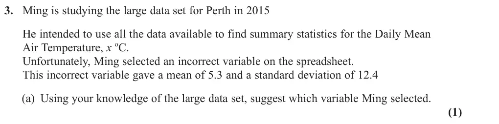
It is encouraging to see most students now attempting the question on the large data set and a growing familiarity with it. In part (a) many wrote down rainfall or windspeed but other quantitative variables such as hours of sunshine or maximum wind gust were sometimes seen but these are not variables available for overseas locations. Some students gave answers like “trace” or “outlier” which have appeared in previous papers but had no relevance to this question. Part (b) was a
Common mistakes
rainfall (or mean windspeed)
hours of sunshine and gusts are not recorded for overseas locations
"trace" or "outlier" irrelevant here
June 2024 · Paper 3 (Statistics) · Q3(b)3 marks
Mark scheme (whole question; this part is marked with the orange bar)
Examiner's comment
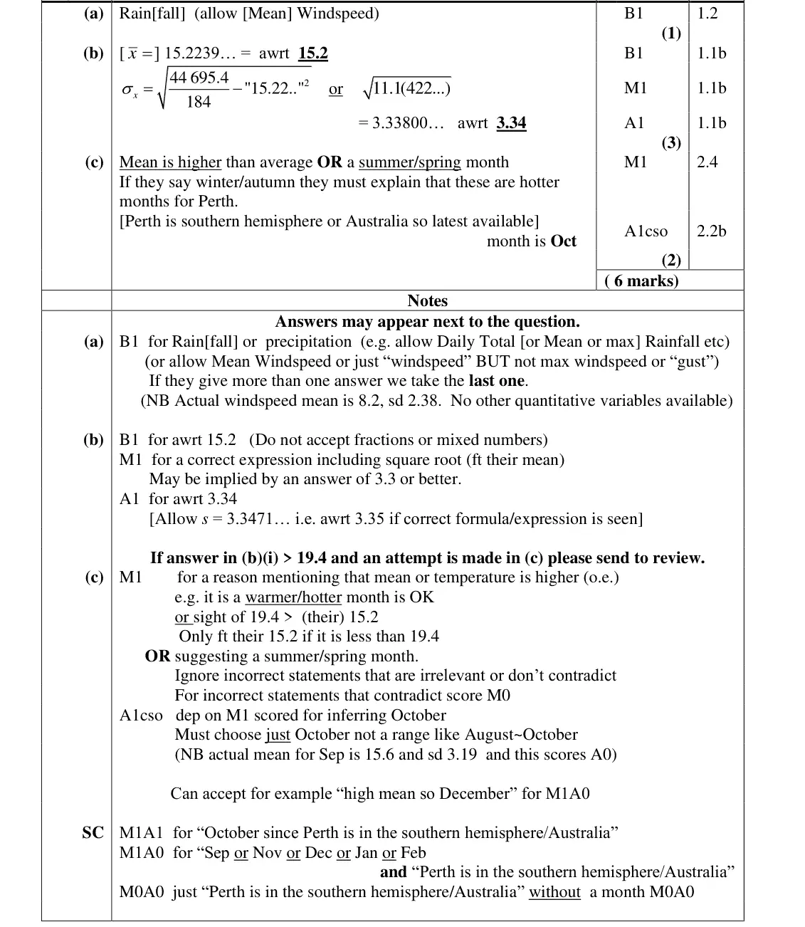
It is encouraging to see most students now attempting the question on the large data set and a growing familiarity with it. appeared in previous papers but had no relevance to this question. Part (b) was a straightforward calculation and was accessible to all the students. Almost everyone scored the mark for the mean and most had a correct expression for the standard deviation, but some used their rounded value of 15.2 for the mean and this meant that their final answer for the standard deviation was not accurate to 3 significant figures. A few students omitted the square root sign or forgot to square the mean. The final part of the question required students to know that Perth on the large data set was in
Common mistakes
mean 2801.2/184 = 15.2
sd = √(44695.4/184 − mean²) = 3.34
use the unrounded mean
remember to square the mean and take the square root
June 2024 · Paper 3 (Statistics) · Q3(c)2 marks
Mark scheme (whole question; this part is marked with the orange bar)
Examiner's comment
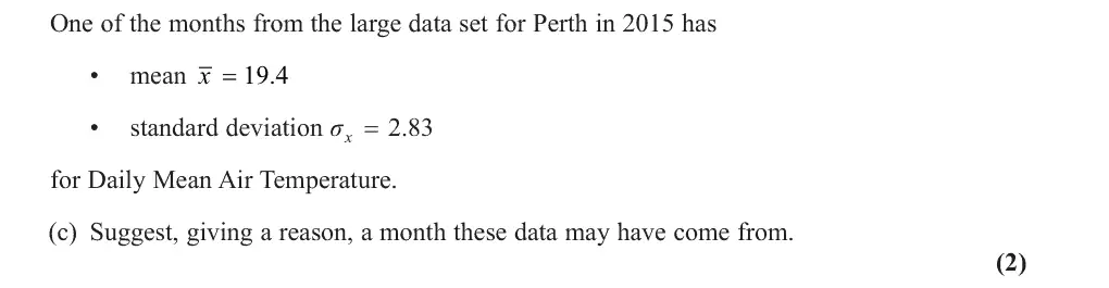
It is encouraging to see most students now attempting the question on the large data set and a growing familiarity with it. The final part of the question required students to know that Perth on the large data set was in the southern hemisphere and therefore the warmer months would be during our autumn and winter. They were told that the mean air temperature for the month in question was 19.4 and needed to observe that this was larger than the overall mean of 15.2 for the 6 months of the large data set. Using their knowledge that the large data set only covers the months from May to October they could then infer that the month in question was October. Many were able to identify that the month to be identified was a warmer month (and scored the first mark) but then suggested an answer such as November or December which of course are not available in the large data set. It was sometimes difficult to know whether a candidate was using “summer” to simply refer to the months from June to August or referring to the warmest months of the year in Perth, often an example month was given which helped clarify what the student meant.
Common mistakes
19.4 is above the overall mean 15.2 so a warmer month
Perth is in the southern hemisphere and the data set covers May–October, so October
November/December are not in the data set
June 2023 · AS Paper 2 (Statistics) · Q1(a)2 marks
Mark scheme (whole question; this part is marked with the orange bar)
Examiner's comment
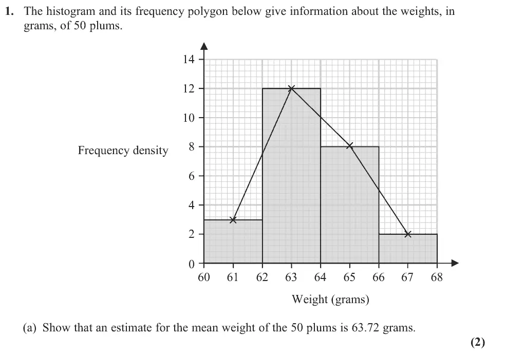
Part (a) was a generally successful start to the paper with the vast majority of students able to show sufficient calculations to arrive at the given mean. A few students opted to use the upper class boundary in their calculation. On some occasions 3186 50 was written with no supporting evidence. Some students misunderstood the demand and attempted to use interpolation to find the median instead of the mean.
Common mistakes
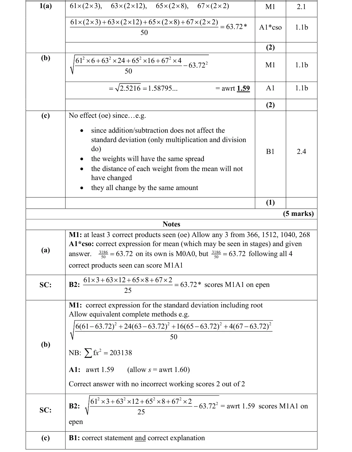
read the histogram: frequency = frequency density × class width 2 (3, 12, 8, 2 doubled to 6, 24, 16, 4)
use midpoints 61, 63, 65, 67, not upper boundaries
3186/50 alone with no products scores 0
some found the median instead
June 2023 · AS Paper 2 (Statistics) · Q1(b)2 marks
Mark scheme (whole question; this part is marked with the orange bar)
Examiner's comment
On the whole part (b) was also well attempted. A common error remains that students confuse ∑𝑓𝑥2 with (∑𝑓𝑥)2.
Common mistakes
sd = √(Σfx²/50 − 63.72²) with Σfx² = 203138 gives 1.59 (s = 1.60 allowed)
confusing Σfx² with (Σfx)²
June 2023 · AS Paper 2 (Statistics) · Q1(c)1 mark
Mark scheme (whole question; this part is marked with the orange bar)
Examiner's comment
Many students were able to score the mark in part (c) as they gave an acceptable explanation why the standard deviation does not change. Some said it did not change but provided no supporting explanation whilst others believed the change in the mean would affect the standard deviation.
Common mistakes
no effect: subtracting 5 g from every weight does not change the spread (only multiplying/dividing does)
a reason is needed
some thought the change in mean changes the sd
June 2023 · AS Paper 2 (Statistics) · Q2(d)1 mark
Mark scheme (whole question; this part is marked with the orange bar)
Examiner's comment
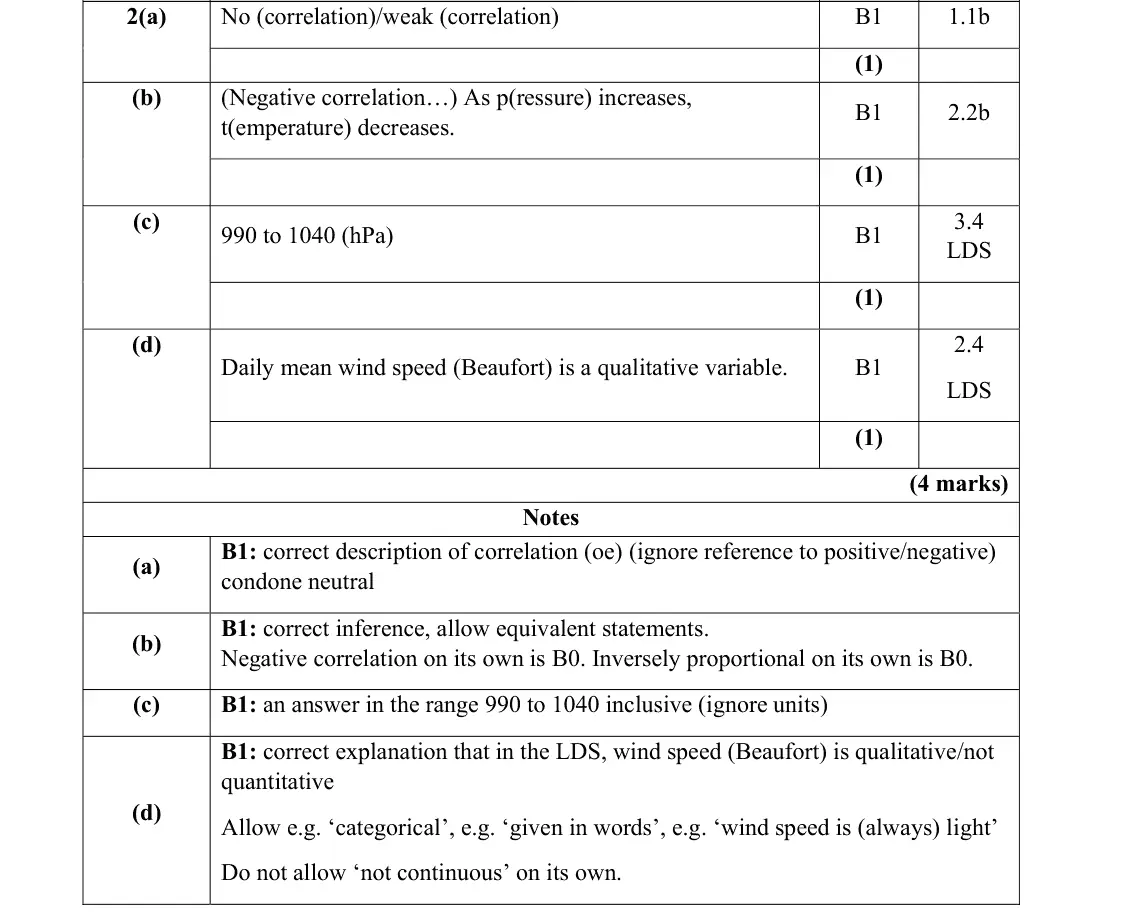
but due to parts (c) and (d) requiring familiarity with the large data set, only a small minority of students scored full marks here. Most students successfully answered part (a) with a correct interpretation of a lack of standard in parts (c) and (d) was poor. Most students guessed an answer to part (c) but very few were able to give an answer in the correct range. In part (d), the students often described the location of Beijing as a factor or repeated an answer given in previous examination series rather than comment on the Beaufort Conversion being qualitative data. It was clear the students who had studied the large data set as their answers had a concise explanation.
Common mistakes
Daily Mean Wind Speed (Beaufort Conversion) is qualitative/categorical (given in words)
"not continuous" alone not accepted
location of Beijing is not a reason
June 2023 · Paper 3 (Statistics) · Q3(a)2 marks
Mark scheme (whole question; this part is marked with the orange bar)
Examiner's comment
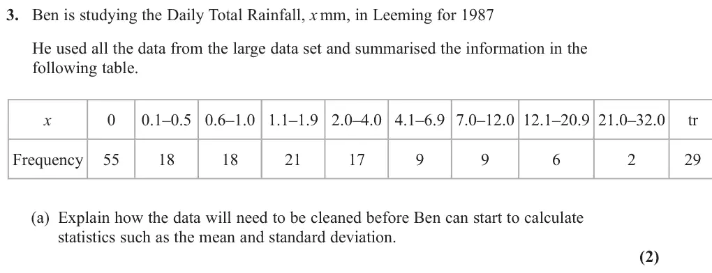
Once again the large data set aspects of this question caused problems for some students but most scored some marks here. In part (a) a few responses simply quoted standard textbook answers about cleaning data by removing outliers and others were distracted by the class intervals for the data. Many though did realise that the “tr” values needed attention but a number didn’t seem to realise that trace entries had a value between 0 and 0.05 and therefore removing them would have a big effect on the calculations Ben wanted to carry out. Those that did appreciate the value of the “tr” usually suggested a suitable numerical value (usually 0) to replace them with and scored both marks.
Common mistakes
tr (trace) means less than 0.05 mm: replace with a numerical value such as 0 or 0.025, do not remove
removing outliers or equalising class widths is not cleaning here
June 2023 · Paper 3 (Statistics) · Q3(b)3 marks
Mark scheme (whole question; this part is marked with the orange bar)
Examiner's comment
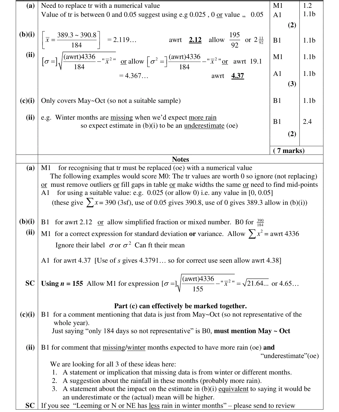
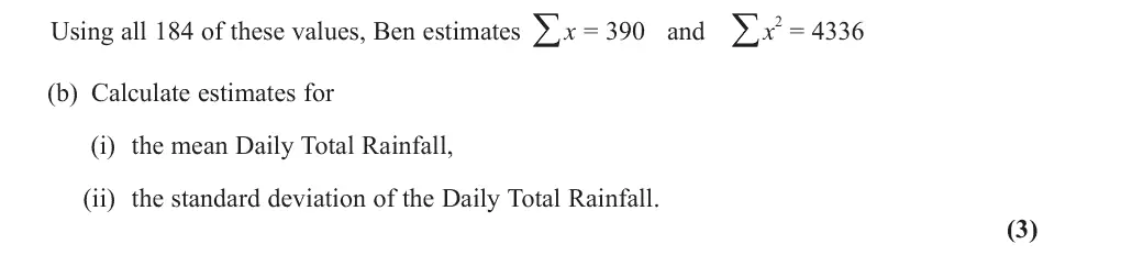
Once again the large data set aspects of this question caused problems for some students but most scored some marks here. Part (b) was, unsurprisingly, answered very well with many scoring full marks. A few lost marks for truncating rather than rounding their answers for example 2.11 in (i) whilst others were convinced that the “tr” values should have been removed and had a denominator of 155 despite the question telling them that all 184 values were used. It is still surprising to see a small number of students using a denominator of 9 or 10 (the number of classes in the table) and a slightly larger proportion who couldn’t use the standard deviation formula, given in the formula booklet, correctly. It was encouraging to see a good number of students demonstrating some familiarity with the large data set and scoring some marks in part (c). In (i) we were simply looking for
Common mistakes
use all 184 values (not 155 or the number of classes)
sd = √(Σx²/n − mean²) = 4.37
round, do not truncate (2.12 not 2.11)
June 2023 · Paper 3 (Statistics) · Q3(c)2 marks
Mark scheme (whole question; this part is marked with the orange bar)
Examiner's comment
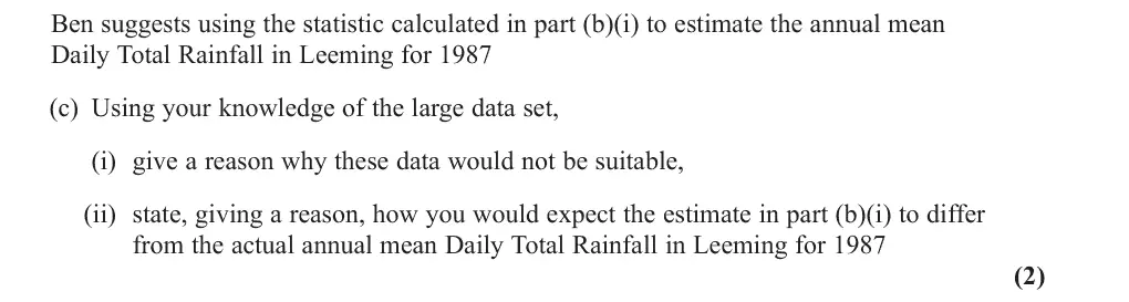
Once again the large data set aspects of this question caused problems for some students but most scored some marks here. the large data set and scoring some marks in part (c). In (i) we were simply looking for an awareness that because the large data set only had data for May to October this would not be representative of the whole population. Some demonstrated a lack of understanding of the principle of using a sample to make inferences by stating that 184 days was not a sufficiently large sample to represent the weather for the whole year. In this case the problem was not the sample size but the fact that the sample was not representative. In (ii) even some of those who had failed to mention May to October in (i) were able to score here by stating that because the missing months were in winter and they expected more rainfall then, the actual mean would be higher. The great storm of October 1987 featured in many incorrect answers to part (c).
Common mistakes
the large data set only covers May to October, so not representative
"184 days is too small a sample" scores B0
winter months are wetter so (b)(i) is an underestimate
the October 1987 storm is not the point
June 2023 · Paper 3 (Statistics) · Q6(a)2 marks
Mark scheme (whole question; this part is marked with the orange bar)
Examiner's comment
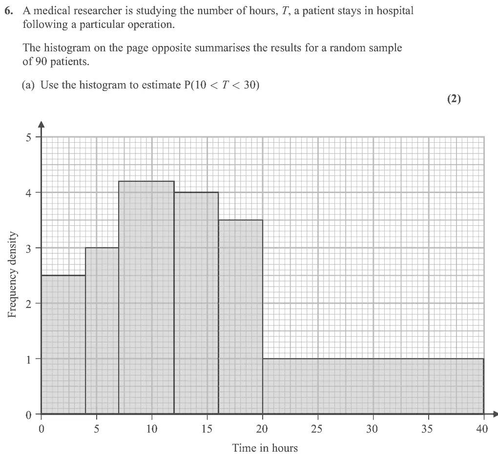
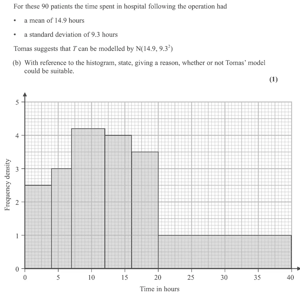
This question also proved to be quite challenging. In part (a) most students could use the histogram to calculate the number of patients spending between 10 and 30 hours in hospital but many failed to convert this to a probability by dividing by 90. Some students tried using small squares, but errors were often made and a divisor of 1600 not 1800 was often seen. Part (b) though was not The first part of (e) was often answered well and some realised that the answer to part (c) could be used to answer (e)(ii) but some tried using n = 10 and 30 and others stopped after find an estimate for the number of patients as 53.1 and failed to complete the question to find the required probability. In part (f) only a small number of candidates realised that
Common mistakes
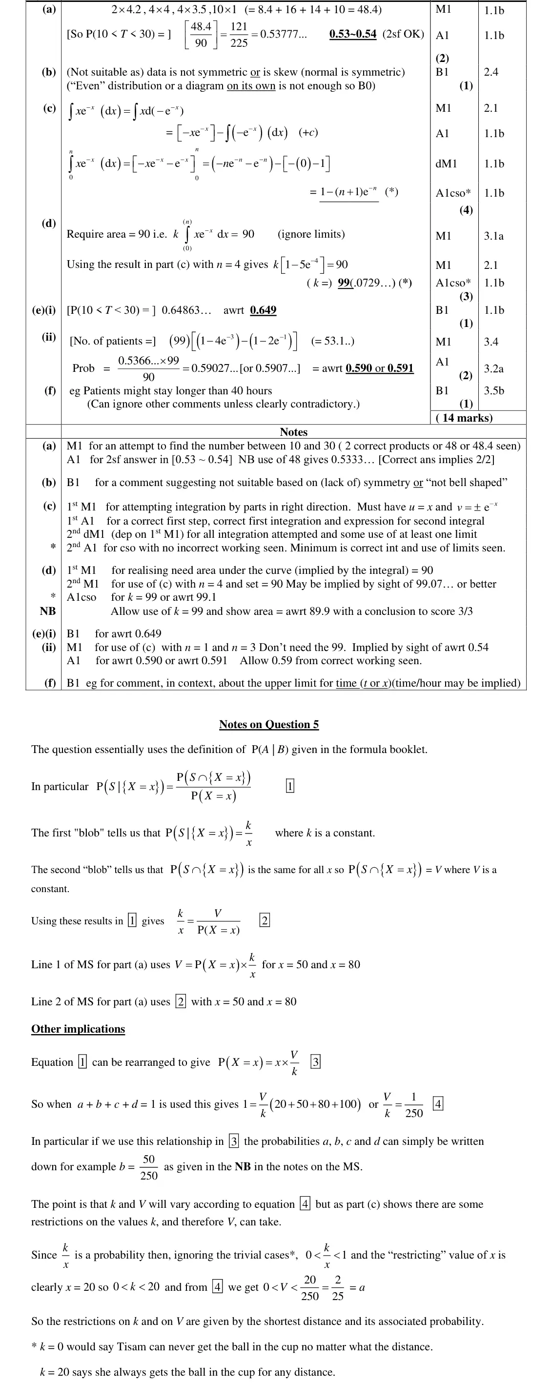
frequency = class width × frequency density (48.4 patients)
divide by 90 for a probability
counting small squares with divisor 1600 instead of 1800
June 2023 · Paper 3 (Statistics) · Q6(b)1 mark
Mark scheme (whole question; this part is marked with the orange bar)
Examiner's comment
This question also proved to be quite challenging. often made and a divisor of 1600 not 1800 was often seen. Part (b) though was not answered so well. Some did explain that the histogram was not symmetric or was skewed and so a normal distribution wouldn’t be suitable. Some focussed on the continuous nature of the variable and thought it was therefore suitable whilst others thought that T was discrete and therefore a normal wasn’t suitable. The question wanted reference to the histogram and there was no expectation or requirement to find probabilities from the normal distribution nor compare the mean of the data with 14.9 If further calculations were expected these would be asked for and reflected in the mark allocation. Many students were able to use integration by parts correctly to establish the result in part
Common mistakes
histogram is skewed/not symmetric but the normal is symmetric
arguments about T being continuous or discrete score B0
no calculation expected
June 2023 · Paper 3 (Statistics) · Q6(c)4 marks
Mark scheme (whole question; this part is marked with the orange bar)
Examiner's comment
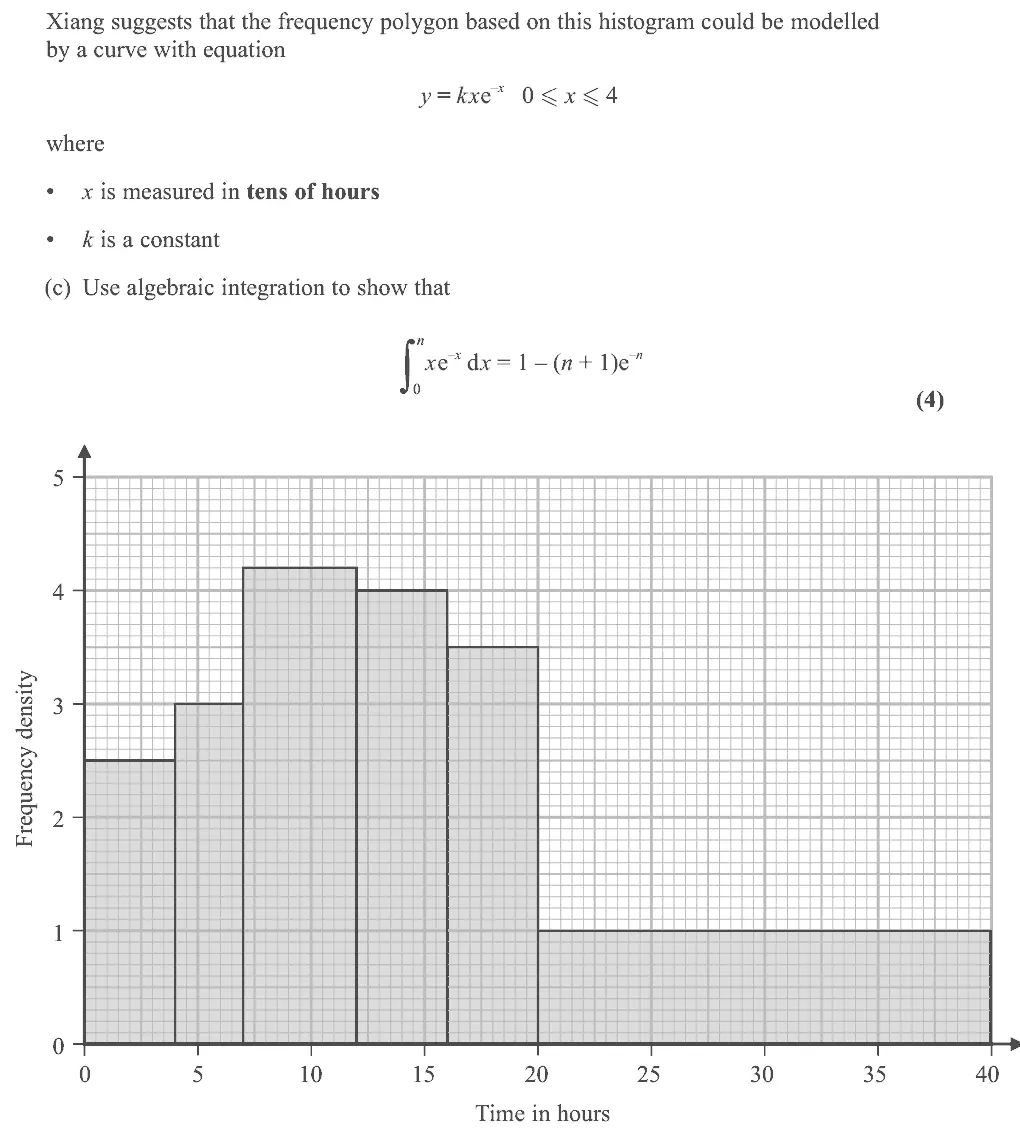
This question also proved to be quite challenging. (c). Some started the wrong way around (using u = e – x) and soon realised they were not heading for the given answer and there was some muddling over the signs when applying the limits. Part (d) was not answered so well with only a minority of students realising to apply the answer to part (c) though some used n = 40 rather than n = 4. The first part of (e) was often answered well and some realised that the answer to part (c) could be used to answer (e)(ii) but some tried using n = 10 and 30 and others stopped after find an estimate for the number of patients as 53.1 and failed to complete the question to find the required probability. In part (f) only a small number of candidates realised that
Common mistakes
integration by parts with u = x, dv/dx = e^(−x) (starting with u = e^(−x) fails)
sign errors when applying the limits
June 2023 · Paper 3 (Statistics) · Q6(d)3 marks
Mark scheme (whole question; this part is marked with the orange bar)
Examiner's comment
This question also proved to be quite challenging. the limits. Part (d) was not answered so well with only a minority of students realising that the area under the curve should equal 90. Those who did realise this were often able to apply the answer to part (c) though some used n = 40 rather than n = 4.
Common mistakes
total area under the curve = 90 patients
use (c) with n = 4 (x in tens of hours, not n = 40)
June 2023 · Paper 3 (Statistics) · Q6(e)(ii)2 marks
Mark scheme (whole question; this part is marked with the orange bar)
Examiner's comment
This question also proved to be quite challenging.
Common mistakes
use (c) with n = 3 and n = 1 (not 30 and 10) to get 53.1 patients, then divide by 90 for the probability 0.590
June 2023 · Paper 3 (Statistics) · Q6(f)1 mark
Mark scheme (whole question; this part is marked with the orange bar)
Examiner's comment
This question also proved to be quite challenging. find the required probability. In part (f) only a small number of candidates realised that the fact that some patients might stay longer than 40 hours was a limitation of the model. Others did not give any context in their answers or discussed the shape of the curve without considering the stated upper limit.
Common mistakes
model only defined for 0 ≤ x ≤ 4, so patients staying longer than 40 hours are not covered
answer must be in context, not about the shape of the curve
June 2022 · AS Paper 2 (Statistics) · Q3(a)4 marks
Mark scheme (whole question; this part is marked with the orange bar)
Examiner's comment
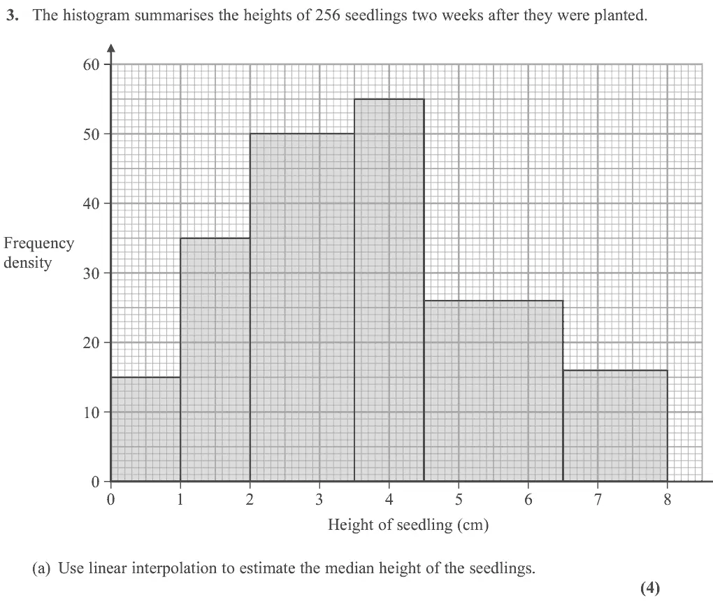
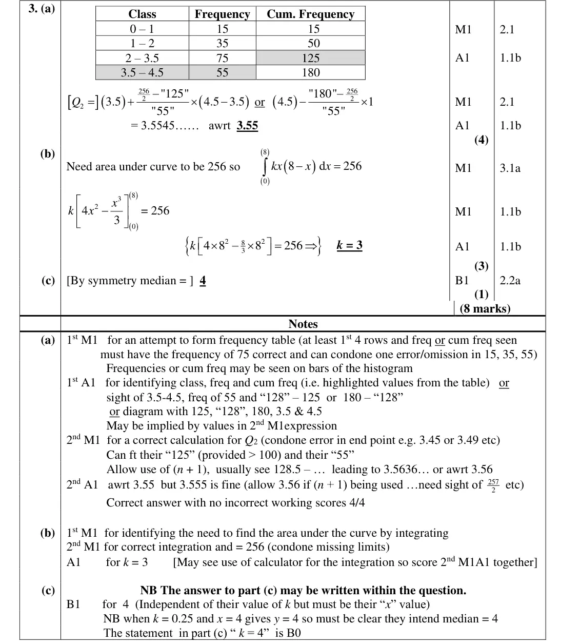
Part (a) should have been familiar territory for candidates and most did manage to list the frequencies for each of the bars though, rather disappointingly, nearly a quarter of candidates could not do this successfully with a common incorrect answer of 50 rather than 75 being recorded for the bar between 2 and 3.5 Those who did understand this important feature of histograms often went on to use linear interpolation correctly to find the median. (a).
Common mistakes
area = frequency: frequencies 15, 35, 75, 55 (common error 50 for the 2 to 3.5 bar, reading the height not the area)
median class 3.5 to 4.5
3.5 + (128 − 125)/55 × 1 = 3.55
June 2022 · AS Paper 2 (Statistics) · Q3(b)3 marks
Mark scheme (whole question; this part is marked with the orange bar)
Examiner's comment
Part (b) sadly defeated almost all candidates. This was the first time we had attempted to assess the part of the specification dealing with “connect(ion) (of histograms) to probability distributions” (section 2.1). A small minority of candidates realised they needed to integrate and set the area under the curve to 256 and they often went onto achieve the correct value of k but most attempts involved differentiating the curve or solving a quadratic equation and made no progress. A few could use the symmetry of the model in part (c) to write down the median but most were completely lost after part
Common mistakes
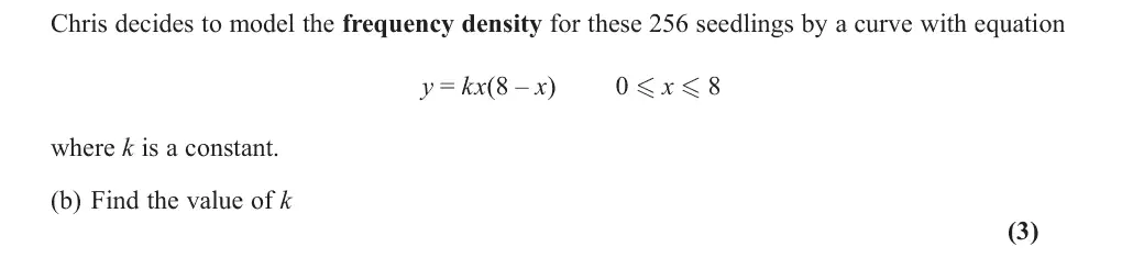
area under the frequency-density curve = total frequency 256, so integrate kx(8 − x) from 0 to 8
k = 3
most differentiated or solved a quadratic instead
June 2022 · AS Paper 2 (Statistics) · Q3(c)1 mark
Mark scheme (whole question; this part is marked with the orange bar)
Examiner's comment
symmetry of the model in part (c) to write down the median but most were completely lost after part
Common mistakes
curve is symmetric about x = 4 so median = 4
"k = 4" scores 0
June 2022 · AS Paper 2 (Statistics) · Q4(a)1 mark
Mark scheme (whole question; this part is marked with the orange bar)
Examiner's comment
Although a few students simply left this question blank most had a go though only about a quarter scored either of the marks. The median was the most successfully answered with 1000 being a common acceptable value. Selecting a suitable value for the range was more challenging with most responses being far too large. Although the specification requires students to be “familiar” with the large data set, for this sitting it is understandable that many would not have had as much time for familiarisation as would be desirable.
Common mistakes
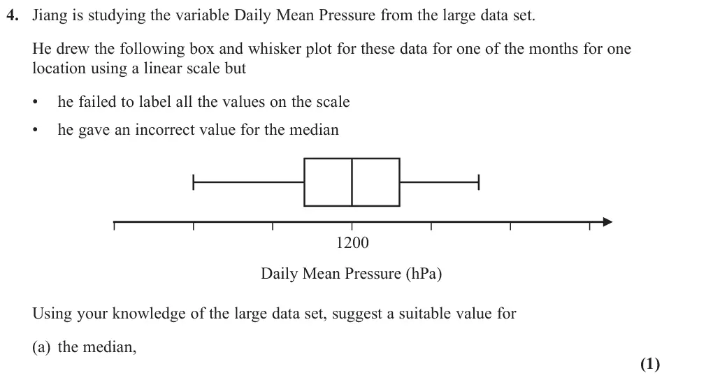
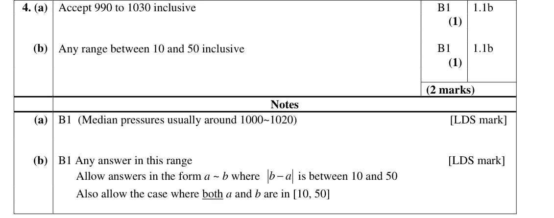
LDS daily mean pressure is around 1000 to 1020 hPa (accept 990 to 1030), not 1200
June 2022 · AS Paper 2 (Statistics) · Q4(b)1 mark
Mark scheme (whole question; this part is marked with the orange bar)
Examiner's comment
Although a few students simply left this question blank most had a go though only about a quarter scored either of the marks. The median was the most successfully answered with 1000 being a common acceptable value. Selecting a suitable value for the range was more challenging with most responses being far too large. Although the specification requires students to be “familiar” with the large data set, for this sitting it is understandable that many would not have had as much time for familiarisation as would be desirable.
Common mistakes
range of daily mean pressure in a month is about 10 to 50 hPa
most answers far too large
June 2022 · Paper 3 (Statistics) · Q3(a)1 mark
Mark scheme (whole question; this part is marked with the orange bar)
Examiner's comment
Part (a) tested knowledge of the data set. Some students were able to identify tr or trace as the required answer, but many displayed their lack of knowledge of the data set, with n/a being a typical wrong answer, or 0 or 0.025. Many students gave no answer of any sort and there were a few nonsensical or confused answers such as explaining how the rainfall might be collected (a particular favourite being ‘with a bucket and ruler’) or how it might be recorded (in an excel spreadsheet).
Common mistakes
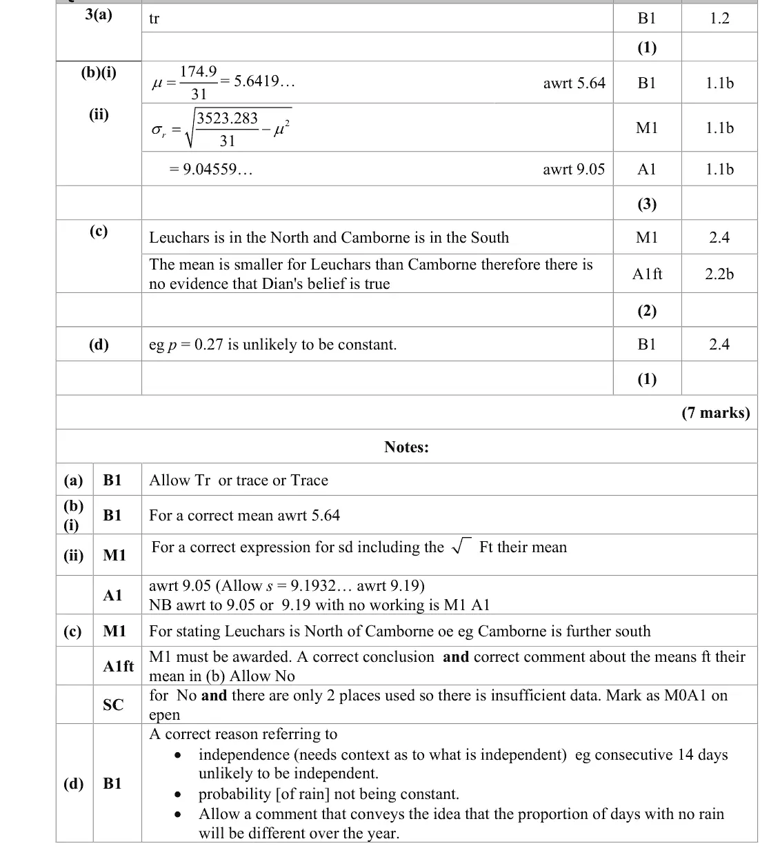
tr (trace)
n/a, 0 or 0.025 are wrong
June 2022 · Paper 3 (Statistics) · Q3(b)3 marks
Mark scheme (whole question; this part is marked with the orange bar)
Examiner's comment
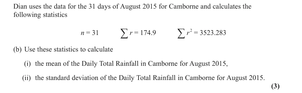
The vast majority of students were able to find the mean correctly in Part (b). Mistakes if any in (i) tended to be rounding the answer to 5.6 without previously showing a more accurate answer, hence losing the single mark. A few students showed the calculation without evaluating it. Disturbingly there was a tiny minority who seemed to have formulae involving square root signs etc. It is disappointing to see evidence of students studying statistics at advanced level who still do not know how to calculate a mean. There were more errors (ii) although well answered by the majority. Errors tended to be missing the square root in their expression for the standard deviation giving the variance as the final answer, with students believing this to be the standard deviation; subtracting the mean rather than the square of the mean premature approximation of the mean leading to inaccurate final answers and giving the answer to 2sf or an even lesser degree of accuracy. A small number of students gave an answer with no working and were then at the mercy of having obtained a sufficiently accurate answer or risk losing these relatively easy marks. The calculation and use of 𝑆𝑆𝑥𝑥𝑥𝑥 was seen occasionally.
do not leave the variance or subtract the mean instead of its square
avoid premature rounding
June 2022 · Paper 3 (Statistics) · Q3(c)2 marks
Mark scheme (whole question; this part is marked with the orange bar)
Examiner's comment
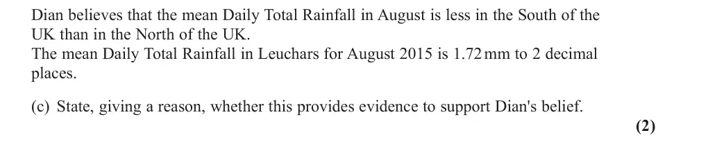
Part (c) proved to be more problematic. Many students lacked knowledge of the LDS and did not know the relative geographical locations of Camborne and Leuchars within the UK. As such, a significant number of students made the incorrect assumption that Leuchars is in the South and Camborne is in the North. However, when students were able to locate the relative positions of the two places correctly, they were generally able to draw the correct conclusion, resulting from comparing the mean rainfall between the two places. The main errors included • not making reference to the relative positions of the two locations in their answer e.g. stating that Camborne was in the South with no reference to the relative position of Leuchars, • not making any statements about either of the geographical locations at all and only compared means, with responses such as: no, as the mean is less in Leuchars than in Camborne. • not drawing the correct conclusion after correctly comparing locations and means • not stating any conclusion. • incorrectly comparing standard deviations rather than means.
Common mistakes
Leuchars is north of Camborne (many got this the wrong way round)
Leuchars has the smaller mean so no evidence for the belief
compare means, not standard deviations
Oct 2021 · AS Paper 2 (Statistics) · Q2(a)3 marksEasy
Mark scheme (whole question; this part is marked with the orange bar)
Examiner's comment
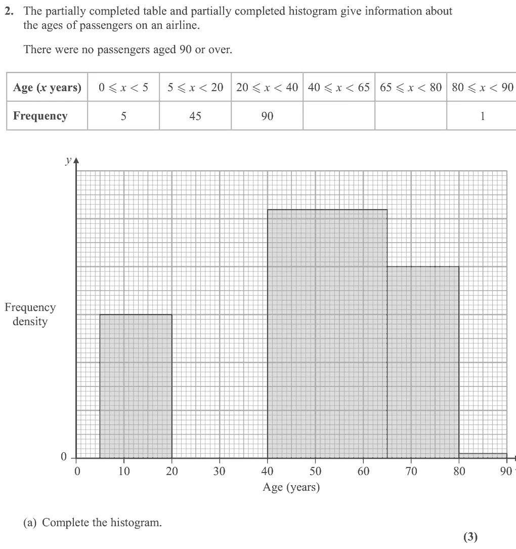
The response to this question on histograms was much better than in previous series with over 50% scoring 7 or more marks. Most managed to complete at least one of the bars of the histogram correctly but a
Common mistakes
find the scale from the [5, 20) bar: fd = 45/15 = 3
bars for [0, 5) at fd 1 and [20, 40) at fd 4.5
area represents frequency
Oct 2021 · AS Paper 2 (Statistics) · Q2(b)4 marksEasy
Mark scheme (whole question; this part is marked with the orange bar)
Examiner's comment
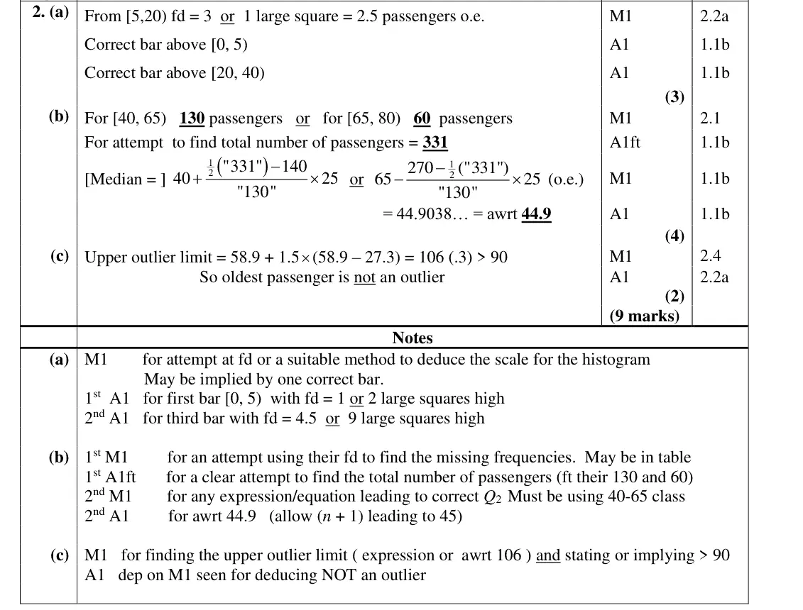
The response to this question on histograms was much better than in previous series with over 50% scoring 7 or more marks. Most managed to complete at least one of the bars of the histogram correctly but a sizeable minority did not make any progress at all here. In part (b) many were able to complete the table correctly and find the total number of passengers. They could often go on to find the median but there were some errors in class boundaries and a fair number of very confused attempts. In part (c) most were able to
Common mistakes
read fd from the histogram to get 130 and 60, total 331
median from the 40–65 class: 40 + (165.5 − 140)/130 × 25 = 44.9
errors in class boundaries
Oct 2021 · AS Paper 2 (Statistics) · Q2(c)2 marksEasy
Mark scheme (whole question; this part is marked with the orange bar)
Examiner's comment
The response to this question on histograms was much better than in previous series with over 50% scoring 7 or more marks. Most managed to complete at least one of the bars of the histogram correctly but a some errors in class boundaries and a fair number of very confused attempts. In part (c) most were able to find the upper outlier limit but some were not able to explain clearly why they could then deduce that none of the passengers were outliers. We required a clear statement that none of the passengers were over 90 and 90 was less than this limit so there were no outliers.
Common mistakes
upper limit 58.9 + 1.5 × 31.6 = 106.3
must state that no passenger is 90 or over and 90 < 106 so the oldest is not an outlier
Oct 2021 · Paper 3 (Statistics) · Q3(a)1 markEasy
Mark scheme (whole question; this part is marked with the orange bar)
Examiner's comment
Although this question involved familiarisation with the large data set nearly 70% scored 3 or more marks here. Many students knew the units used for Daily Mean Pressure (or wrote “Pascals” which was allowed).
Common mistakes
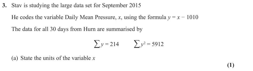
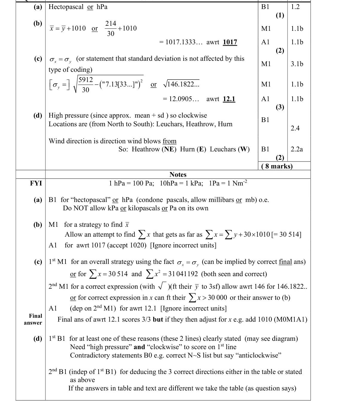
Daily Mean Pressure is in hectopascals (hPa)
kPa or Pa alone not accepted
Oct 2021 · Paper 3 (Statistics) · Q3(b)2 marksEasy
Mark scheme (whole question; this part is marked with the orange bar)
Examiner's comment
Although this question involved familiarisation with the large data set nearly 70% scored 3 or more marks here. Many students knew the units used for Daily Mean Pressure (or wrote “Pascals” which was allowed). The coding caused problems for many in part (b) finding y was easy enough but then adding the 1010 seemed to elude a great number of the candidates. Another frequently seen error was to add 1010 to Σy leading to the common wrong answer of 40.8. Part (c) was the most successful part with many correct
Common mistakes
coding: x̄ = ȳ + 1010 = 214/30 + 1010 = 1017
adding 1010 to Σy gives the common wrong 40.8
Oct 2021 · Paper 3 (Statistics) · Q3(c)3 marksEasy
Mark scheme (whole question; this part is marked with the orange bar)
Examiner's comment
Although this question involved familiarisation with the large data set nearly 70% scored 3 or more marks here. Many students knew the units used for Daily Mean Pressure (or wrote “Pascals” which was allowed). leading to the common wrong answer of 40.8. Part (c) was the most successful part with many correct answers seen; sometimes the effect of coding was clearly stated but often, I suspect, it was simply ignored and the correct answer obtained anyway. Occasionally students felt they should add the 1010 on after reaching the correct value of 12.1 and this just lost the first method mark for this part. The final part proved
Common mistakes
σx = σy as coding by subtraction does not change the s.d.
√(5912/30 − 7.133²) = 12.1
do not add 1010 afterwards
Oct 2021 · Paper 3 (Statistics) · Q3(d)2 marksEasy
Mark scheme (whole question; this part is marked with the orange bar)
Examiner's comment
Although this question involved familiarisation with the large data set nearly 70% scored 3 or more marks here. Many students knew the units used for Daily Mean Pressure (or wrote “Pascals” which was allowed). reaching the correct value of 12.1 and this just lost the first method mark for this part. The final part proved challenging. There was evidence that students knew the relative locations of the 3 sites and often they deduced that it was high pressure and therefore the winds circulated clockwise. The major problem though was that students did not seem to appreciate that Cardinal Wind Direction in the large data set gives the direction from which the wind comes. This led to an incorrect allocation of directions in the table, some students were clearly confused by this and felt that the circulation must be anticlockwise and then a correct allocation of wind directions could, of course, be deduced but this lost the first mark. A small percentage of students though did achieve full marks for this question.
Common mistakes
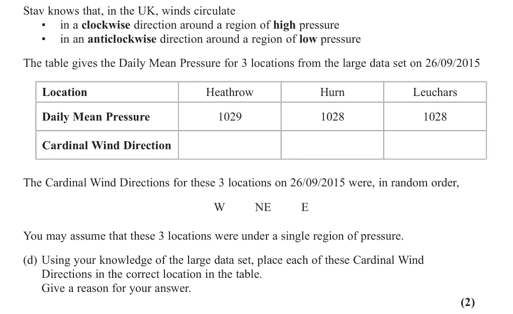
1028–1029 is about mean + s.d., so high pressure and clockwise
locations north to south Leuchars, Heathrow, Hurn
Cardinal Wind Direction is the direction the wind blows FROM: Heathrow NE, Hurn E, Leuchars W
Oct 2020 · AS Paper 2 (Statistics) · Q14 marks
Mark scheme (whole question; this part is marked with the orange bar)
Examiner's comment
This question proved to be quite difficult with the link between area and numbers of students eluding most candidates. Whilst some candidates managed to find the number of students required, they then made no effort at finding the percentage. Working was often confused and lacking organisation which led to many using a mix of "the number of squares in a bar" and "the frequency a bar represents" when finding the total number of students. The other main error was in calculating the heights of the 4 middle bars in terms of small squares. The heights are 8, 4, 12 and 3 but were often given as 10, 5, 15 and 4.
Common mistakes
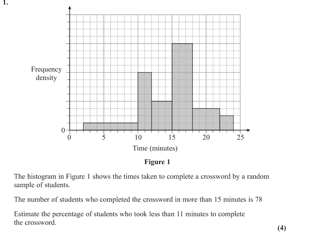
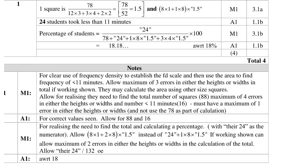
area represents frequency: find 1 square = 78/52 = 1.5 students from the bars above 15 min
bar heights are 8, 4, 12 and 3 small squares (common error 10, 5, 15, 4)
only the part of the 10-12 bar up to 11 counts (24 students)
must go on to divide by the total (132) for a percentage, about 18%
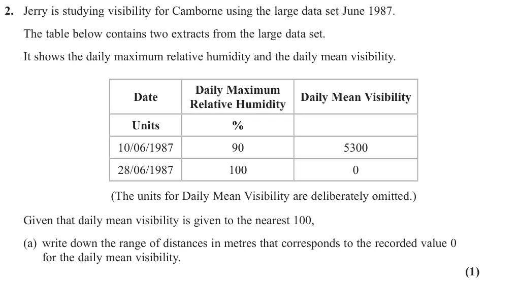
Oct 2020 · AS Paper 2 (Statistics) · Q2(a)1 mark
Mark scheme (whole question; this part is marked with the orange bar)
Examiner's comment
It was clear from the responses seen here that many candidates have little or no experience with the large data set. In part (a) very few students knew that the figures for Daily Mean Visibility are in decametres (Dm). In part (d) a minority of
Common mistakes
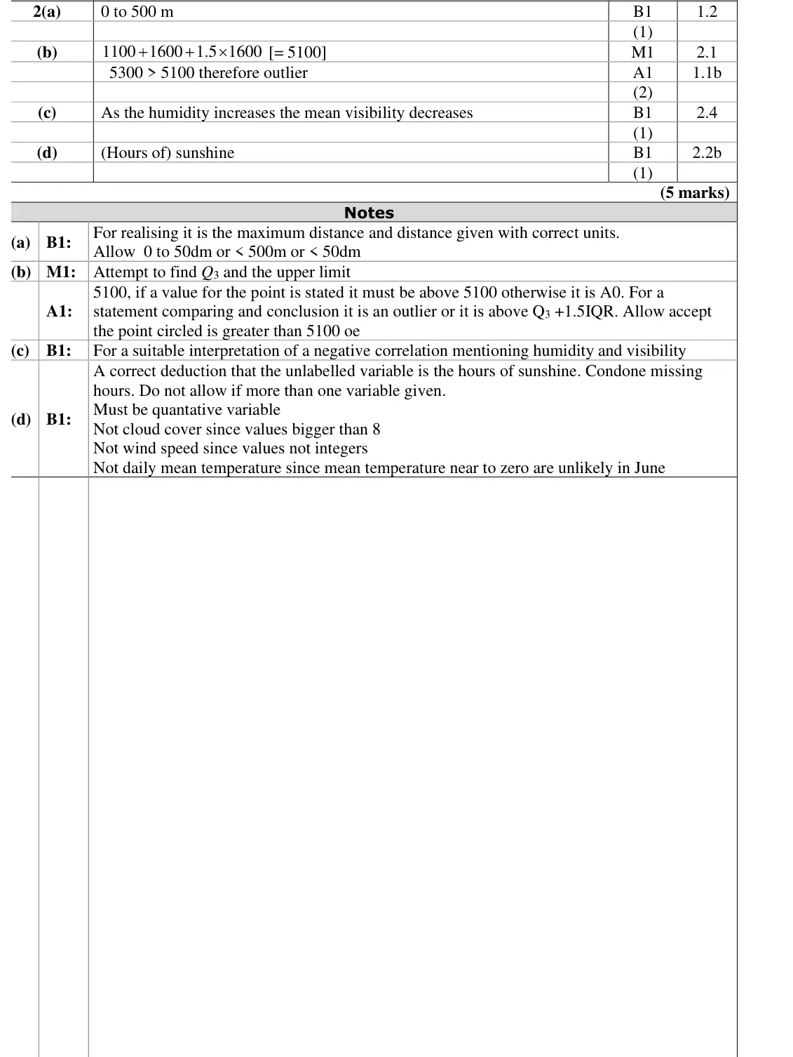
visibility in the large data set is in decametres, so 0 to the nearest 100 dam means 0 to 500 m (or under 50 dam)
very few knew the units
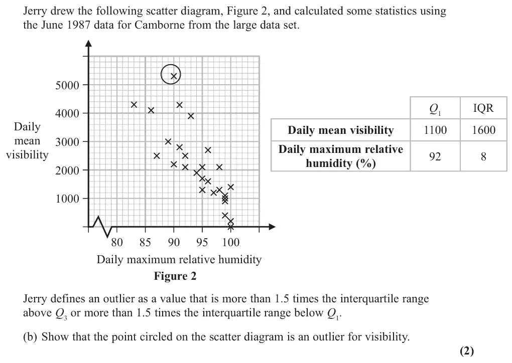
Oct 2020 · AS Paper 2 (Statistics) · Q2(b)2 marks
Mark scheme (whole question; this part is marked with the orange bar)
Examiner's comment
It was clear from the responses seen here that many candidates have little or no In part (b) most candidates who produced an answer were able to gain some marks. The most common mistake was to multiply the LQ by 3 in order to find the UQ. A few candidates calculated the upper boundary correctly, but then failed to make a comparison to finish off their reasoning.
Mark scheme (whole question; this part is marked with the orange bar)
Examiner's comment
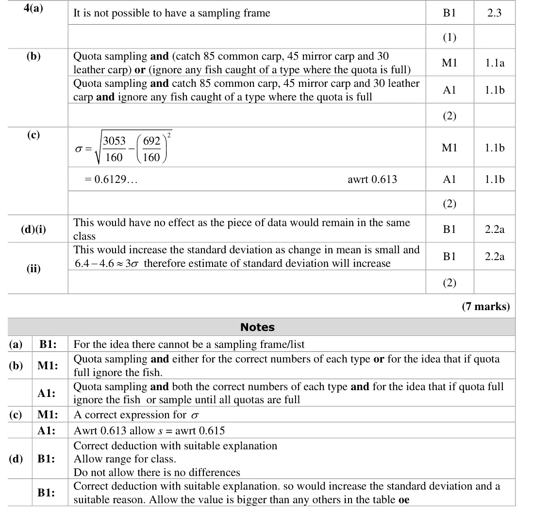
In part (c) far too many candidates (over 35%) had little to no idea of what to do. Those candidates who knew how to calculate the standard deviation often carelessly lost a mark by giving inaccurate answers.
Mark scheme (whole question; this part is marked with the orange bar)
Examiner's comment
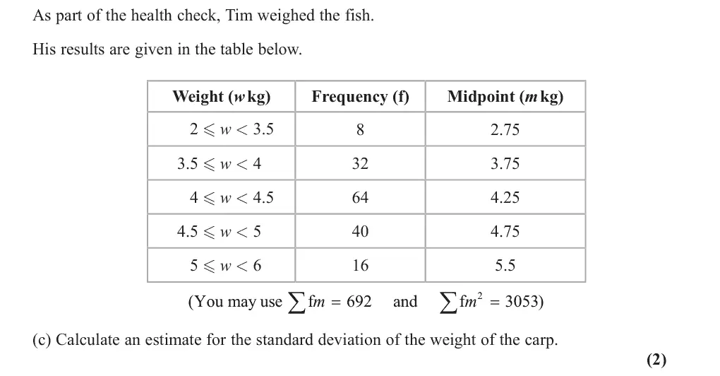
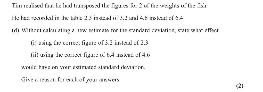
In part (d) it was very rare to see both parts answered correctly. Part(i) was answered the best, but even those who saw that the classes were important could not transfer this idea to the second part. Those candidates who realised the standard deviation will increase in (ii) were rarely able to give a good reason. Many simply stated the range increased but were unable to give an explanation as to why the range increased.
Common mistakes
(i) no effect: 2.3 and 3.2 are in the same class (2 to 3.5)
(ii) sd increases: 6.4 is further from the mean (about 3 sd) than any value / outside the classes
a reason is needed for each
Oct 2020 · Paper 3 (Statistics) · Q3(a)1 mark
Mark scheme (whole question; this part is marked with the orange bar)
Examiner's comment
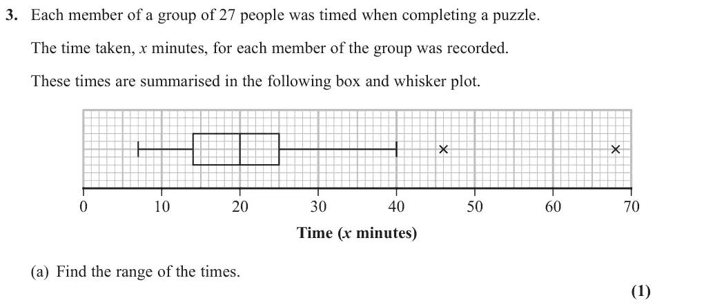
Part (a) should have been an easy start to the question but a surprisingly large number of students gave an answer of 33 by failing to consider the outliers to determine the range.
Common mistakes
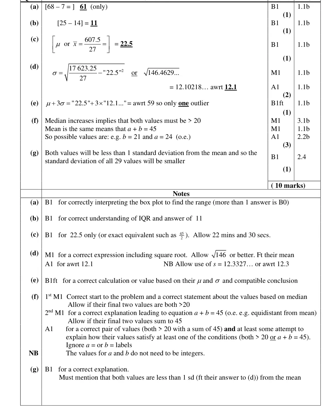
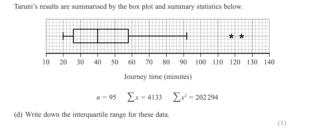
range includes the outliers: 68 − 7 = 61, not 33
Oct 2020 · Paper 3 (Statistics) · Q3(b)1 mark
Mark scheme (whole question; this part is marked with the orange bar)
Examiner's comment
Part (b) though was answered very well and nearly all students answered (c) correctly. The presence of the formula for standard deviation in the formula booklet meant that a good number answered part (d) correctly although occasionally some forgot to take the
Common mistakes
IQR = 25 − 14 = 11
Oct 2020 · Paper 3 (Statistics) · Q3(c)1 mark
Mark scheme (whole question; this part is marked with the orange bar)
Examiner's comment
Part (a) should have been an easy start to the question but a surprisingly large number of students gave an answer of 33 by failing to consider the outliers to determine the range. Part (b) though was answered very well and nearly all students answered (c) correctly. The presence of the formula for standard deviation in the formula booklet meant that a good number answered part (d) correctly although occasionally some forgot to take the square root of failed to square the mean. In (e) most gave a suitable calculation to support their statement that Taruni would identify only 1 outlier. Some candidates used the median of 20 rather than the mean of 22.5 though. The last two parts were more challenging but it was encouraging to see a good number of attempts. Many were able to deduce that because the mean did not change then a + b = 45 but fewer were able to establish that, because the median increases, both values had to be greater than 20. Some did state these two conditions but sadly did not choose suitable values (a = 25 and b = 20 was a common error) for their final answer. In (g) many students stated that the new values would be “close to the mean” but this was not precise enough to ensure that the standard deviation would decrease. Some of the very strongest candidates did realise that because both values were within 1 standard deviation of the mean then they could be sure that the new standard deviation would be smaller. This appreciation that standard deviation represents “average distance from the mean” is clearly not well known.
Common mistakes
mean = 607.5 ÷ 27 = 22.5
Oct 2020 · Paper 3 (Statistics) · Q3(d)2 marks
Mark scheme (whole question; this part is marked with the orange bar)
Examiner's comment
good number answered part (d) correctly although occasionally some forgot to take the square root of failed to square the mean. In (e) most gave a suitable calculation to
Common mistakes
σ = square root of (Σx²/n − mean²) = 12.1
square the mean and take the square root
s = 12.3 also allowed
Oct 2020 · Paper 3 (Statistics) · Q3(e)1 mark
Mark scheme (whole question; this part is marked with the orange bar)
Examiner's comment
square root of failed to square the mean. In (e) most gave a suitable calculation to support their statement that Taruni would identify only 1 outlier. Some candidates used the median of 20 rather than the mean of 22.5 though. The last two parts were more challenging but it was encouraging to see a good number of attempts. Many were able to deduce that because the mean did not change then a + b = 45 but fewer were able to establish that, because the median increases, both values had to be greater than 20. Some did state these two conditions but sadly did not choose suitable values (a = 25 and b = 20 was a common error) for their final answer. In (g) many students stated that the
Common mistakes
mean + 3σ = 22.5 + 3 × 12.1 ≈ 59, so only one outlier (68)
use the mean 22.5, not the median 20
Oct 2020 · Paper 3 (Statistics) · Q3(f)3 marks
Mark scheme (whole question; this part is marked with the orange bar)
Examiner's comment
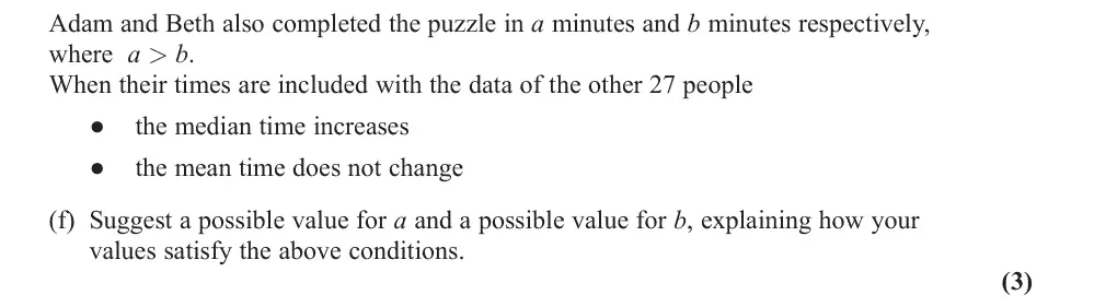
Part (a) should have been an easy start to the question but a surprisingly large number of students gave an answer of 33 by failing to consider the outliers to determine the range. Part (b) though was answered very well and nearly all students answered (c) correctly. The presence of the formula for standard deviation in the formula booklet meant that a good number answered part (d) correctly although occasionally some forgot to take the square root of failed to square the mean. In (e) most gave a suitable calculation to support their statement that Taruni would identify only 1 outlier. Some candidates used the median of 20 rather than the mean of 22.5 though. The last two parts were more challenging but it was encouraging to see a good number of attempts. Many were able to deduce that because the mean did not change then a + b = 45 but fewer were able to establish that, because the median increases, both values had to be greater than 20. Some did state these two conditions but sadly did not choose suitable values (a = 25 and b = 20 was a common error) for their final answer. In (g) many students stated that the new values would be “close to the mean” but this was not precise enough to ensure that the standard deviation would decrease. Some of the very strongest candidates did realise that because both values were within 1 standard deviation of the mean then they could be sure that the new standard deviation would be smaller. This appreciation that standard deviation represents “average distance from the mean” is clearly not well known.
Common mistakes
median increases so both values above 20
mean unchanged so a + b = 45 (e.g. 24 and 21)
a = 25, b = 20 is a common error
explain how the values satisfy both conditions
Oct 2020 · Paper 3 (Statistics) · Q3(g)1 mark
Mark scheme (whole question; this part is marked with the orange bar)
Examiner's comment
b = 20 was a common error) for their final answer. In (g) many students stated that the new values would be “close to the mean” but this was not precise enough to ensure that the standard deviation would decrease. Some of the very strongest candidates did realise that because both values were within 1 standard deviation of the mean then they could be sure that the new standard deviation would be smaller. This appreciation that standard deviation represents “average distance from the mean” is clearly not well known.
Common mistakes
both new values are within 1 standard deviation of the mean, so σ decreases
"close to the mean" is not precise enough
June 2019 · AS Paper 2 (Statistics) · Q4(a)1 mark
Mark scheme (whole question; this part is marked with the orange bar)
Examiner's comment
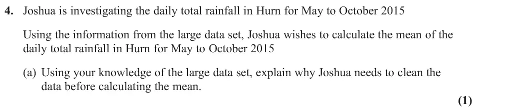
In part (a) most candidates referred to data that was n/a, anomalies or outliers with only a small proportion appreciating that the data set contained trace values for rainfall which needed replacing with numerical values.
Common mistakes
LDS: rainfall includes "tr" (trace, less than 0.05 mm) which must be converted to a number
n/a, missing data or outliers are not the answer
June 2019 · AS Paper 2 (Statistics) · Q4(b)2 marks
Mark scheme (whole question; this part is marked with the orange bar)
Examiner's comment
For part (b) most candidates are familiar with using linear interpolation though slips appear often. Errors with endpoints often resulted in multiplication by 5. Other mistakes included 23 in the denominator or 6 on the numerator. For those using an (n + 1) method, it was not uncommon to see 7.5 being used in the numerator instead of 7.75.
Common mistakes
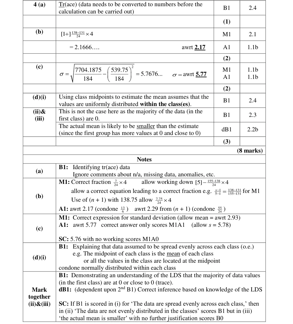
Q3 is the 138th value (184 × ¾)
1 + (138 − 131)/24 × 4 = 2.17
class width 4, not 5
(n + 1) method uses 138.75
June 2019 · AS Paper 2 (Statistics) · Q4(c)2 marks
Mark scheme (whole question; this part is marked with the orange bar)
Examiner's comment
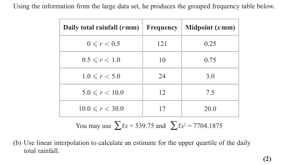
In part (c) most candidates were able to use the given information to arrive at the required result. There are still a large number of candidates who do not work to the appropriate degree of accuracy and 5.8 and 5.76 were often seen. Candidates are encouraged to write down all figures from their calculator before rounding to ensure accuracy marks are scored. Those who did not achieve full marks here often had an incorrect denominator or forgot to include the square root.
Common mistakes
σ = √(7704.1875/184 − (539.75/184)²) = 5.77
n = 184
do not forget the square root
give 3 s.f. (5.8 and 5.76 lose the A mark)
June 2019 · AS Paper 2 (Statistics) · Q4(d)3 marks
Mark scheme (whole question; this part is marked with the orange bar)
Examiner's comment
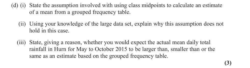
The underlying assumption in part (d)(i) was generally identified but not always with sufficient clarity to gain the mark. Common errors were: ‘data uniformly distributed’ (failing to mention within each class); the average of each class is the midpoint (failing to specify the mean of each class); most of the data is located at the midpoint (failing to identify that the midpoint is assumed to represent all of the data). It was clear from the responses seen here that many candidates have little or no experience with the large data set. In (d)(ii) quite a number referred to the data being based on weather which is unpredictable and that therefore the previous assumption was unrealistic. Good explanations involving the distribution of the bottom class were rare with very few making reference to the majority of data being either 0 or close to 0. Little progress was made in (d)(iii) as many mentioned irrelevancies such as the great storm or the fact that it was during the summer or that the database did not cover a full year. Many did not realise that they were comparing an estimated mean with an actual mean for the same time span and said the actual mean would be higher because the winter months were excluded.
Common mistakes
(i) values are spread evenly within each class (not "data uniformly distributed")
(ii) LDS: most days in the first class have 0 or trace rainfall
(iii) so the actual mean is smaller than the estimate
comparing with winter months or storms is irrelevant
June 2019 · Paper 3 (Statistics) · Q2(a)4 marks
Mark scheme (whole question; this part is marked with the orange bar)
Examiner's comment
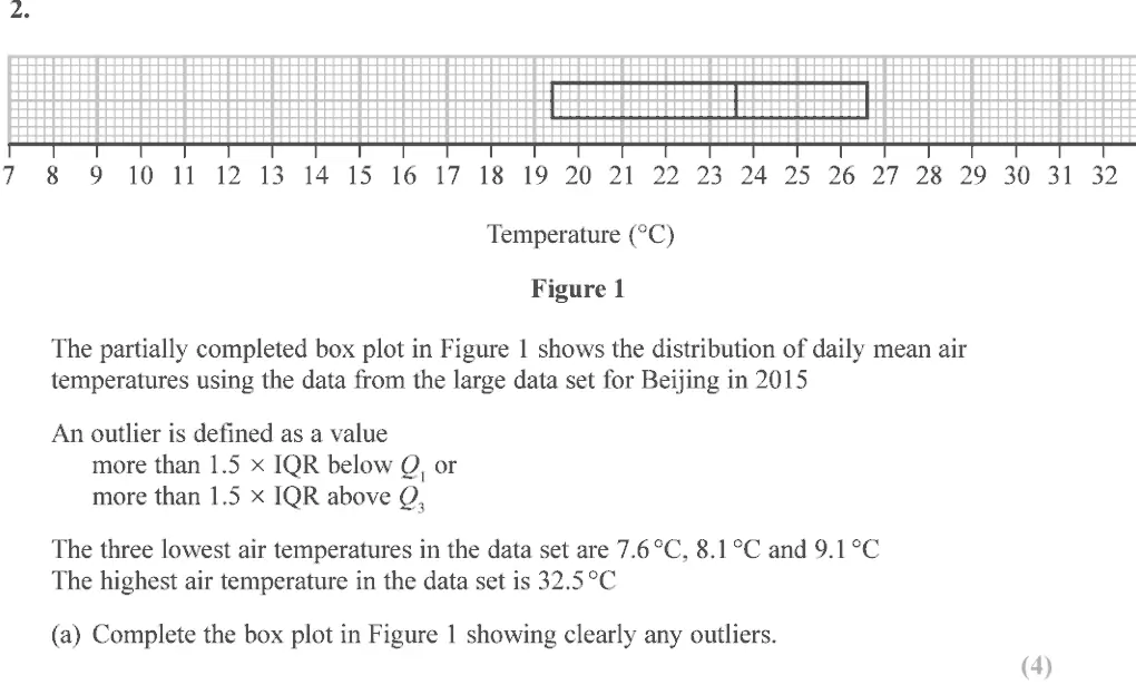
Parts (a), (c) were well attempted by most candidates with part (d) being tackled by more able candidates. Parts (b) and (e) were a problem for those less familiar with the large data set. In (a) most candidates correctly read the quartile values from the diagram to obtain and use the interquartile range to find outlier boundaries. (Where IQR was incorrect it was commonly given as 7.4). Surprisingly there were some inaccuracies in using the formula for outliers even though it was given. Not all candidates showed any working which meant marks could not be awarded if the box plot was not correct. The left hand whisker was commonly drawn to 9.1 (sometimes to 8.6) as required but the right hand whisker was more occasionally incorrect, often extending off the grid instead of stopping at the stated maximum value of 32.5 Usually the two outliers were plotted although they were sometimes omitted by candidates who had shown the correct calculations. Candidates are required to be familiar with the large data set. It was clear from responses in
Common mistakes
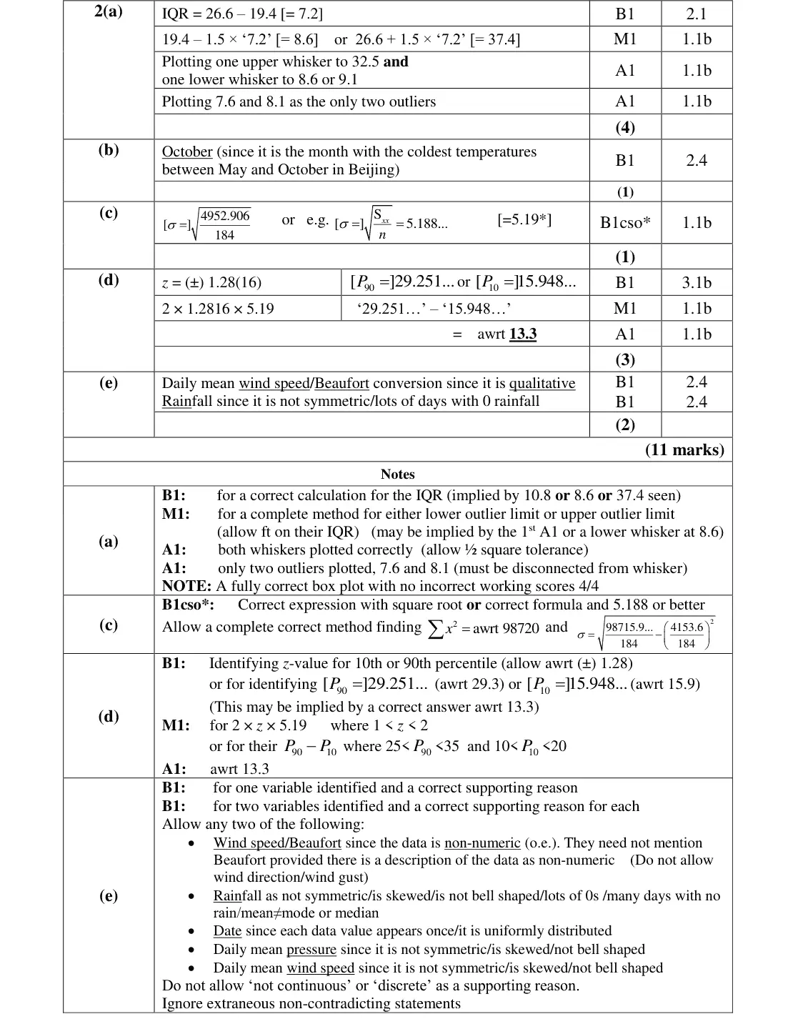
IQR = 26.6 − 19.4 = 7.2
limits 8.6 and 37.4
lower whisker to 8.6 or 9.1, upper whisker to 32.5 (not off the grid)
plot 7.6 and 8.1 as the only outliers
show working
June 2019 · Paper 3 (Statistics) · Q2(b)1 mark
Mark scheme (whole question; this part is marked with the orange bar)
Examiner's comment
candidates. Parts (b) and (e) were a problem for those less familiar with the large data set. part (b) that many were not aware that for all locations the data is for the months of May to October only. Successful candidates often explained that Beijing was in the northern hemisphere and so low outliers for temperature were likely to be for winter, and so October. Some candidates perhaps did not read the question carefully enough and stated two months. S Most candidates scored well in part (c), usually using the given formula. A small xx
Common mistakes
LDS covers May to October only
Beijing is in the northern hemisphere so the coldest month is October
give one month only
June 2019 · Paper 3 (Statistics) · Q2(c)1 mark
Mark scheme (whole question; this part is marked with the orange bar)
Examiner's comment
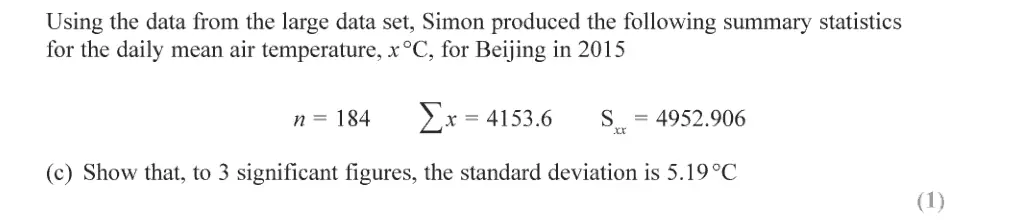
Parts (a), (c) were well attempted by most candidates with part (d) being tackled by more able candidates. Parts (b) and (e) were a problem for those less familiar with the large data set. S Most candidates scored well in part (c), usually using the given formula. A small xx n 2x S to find number appeared unaware of this method instead choosing to work back from , xx to then use in the ‘standard’ formula. Some were successful here although there were a number 2x S to be who mistakenly took the given . Most candidates showed their calculation xx giving the result to at least 4 significant figures so that they could show it rounded to 5.19 The most popular approach in part (d) here seemed to be use of the inverse Normal function
Common mistakes
σ = √(Sxx/n) = √(4952.906/184) = 5.188…
give more than 3 s.f. before rounding
do not treat Sxx as Σx²
June 2019 · Paper 3 (Statistics) · Q2(d)3 marks
Mark scheme (whole question; this part is marked with the orange bar)
Examiner's comment
Parts (a), (c) were well attempted by most candidates with part (d) being tackled by more able candidates. Parts (b) and (e) were a problem for those less familiar with the large data set. The most popular approach in part (d) here seemed to be use of the inverse Normal function on a calculator to find the 10th and 90th percentiles. This was usually successful although many candidates then went no further, hence gaining only the first mark. It was evident that some were not aware of what was meant by interpercentile range; it was not understood that the difference needed to be found (as when finding IQR), some stating a range for x as an inequality (e.g. 15.9 ) with others instead reaching a probability answer of 0.8. Of those 29.3 x continuing to find the IPR some had prematurely rounded both percentile values to 3 significant figures before subtraction, leading to 13.4 as an inaccurate final answer. Candidates need to be encouraged to work with accurate figures, only rounding their final answer. Fewer candidates used the more ‘traditional’ (and longer) approach of standardisation to obtain the percentiles needed, although this was often done successfully.
the range is a difference, not an inequality or 0.8
rounding percentiles early gives 13.4
June 2018 · AS Paper 2 · Q4(a)1 mark
Mark scheme (whole question; this part is marked with the orange bar)
Examiner's comment
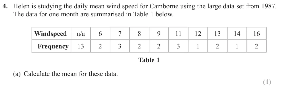
The new specification requires students to be familiar with the large data set and the first part of the question addressed this issue. In part (a) the students needed to realise that n/a in the large data set means that the data for that point was not available and this means that there are only 18 (not 31) pieces of data available. Another skill students are required to have under the new specification is to be able to calculate standard statistics using their calculators. In this case, we expected students to enter the data into their calculator and write down the mean (part (a)) and standard deviation (part
Common mistakes
n/a means data not available, so n = 18 not 31 (treating n/a as 0 gives 5.94)
mean 184/18 = 10.2
use the calculator's statistics mode
June 2018 · AS Paper 2 · Q4(b)2 marks
Mark scheme (whole question; this part is marked with the orange bar)
Examiner's comment
(b)). It was clear that many students were not familiar with this requirement and we often saw several lines of working to derive these results which unfortunately under the new specification cannot receive any marks. A small number of students knew that wind speed was measured in knots but many did not know this.
Common mistakes
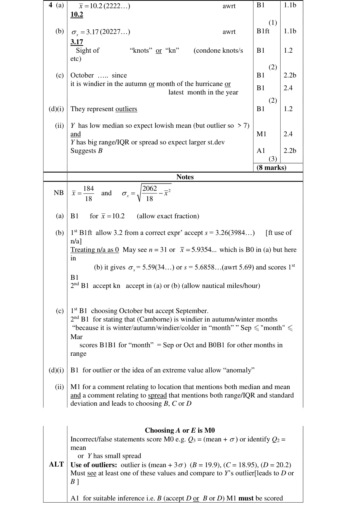
σ = 3.17 (s = 3.26 accepted) from n = 18
units are knots (kn), which many did not know
long hand derivations earn no extra credit
June 2018 · AS Paper 2 · Q4(c)2 marks
Mark scheme (whole question; this part is marked with the orange bar)
Examiner's comment
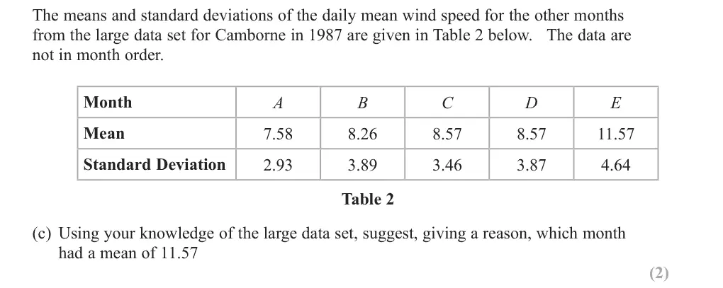
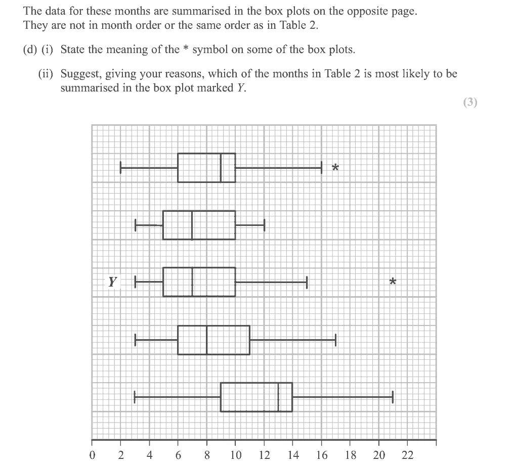
In part (c) there were many good attempts and most students gave a correct response here and in (d)(i) most knew that the * represented an outlier. Part (ii) was very challenging and required some careful thought and inference. Some confused mean with median and assumed that C and D were the 2nd and 3rd box plots in the list since they had the same medians. The intention was that they should identify E as the 5th box plot and A as the 2nd (it has a low mean and standard deviation and clearly has the smallest range on the box plots). Looking at the other 3 they should notice that the range is large and the outlier too would suggest a large standard deviation. The box plot Y has the smallest median of these 3 so a lower mean is suggested which points to B. We were looking for some explanation using correct terminology so we expected references to the mean and median and the standard deviation and a suitable measure of spread from the box plots.
Common mistakes
October (accept September): Camborne is windier in autumn, October 1987 was the month of the hurricane, or it is the latest month in the data
June 2018 · AS Paper 2 · Q4(d)3 marks
Mark scheme (whole question; this part is marked with the orange bar)
Examiner's comment
In part (c) there were many good attempts and most students gave a correct response here and in (d)(i) most knew that the * represented an outlier. Part (ii) was very challenging and required some careful thought and inference. Some confused mean with median and assumed that C and D were the 2nd and 3rd box plots in the list since they had the same medians. The intention was that they should identify E as the 5th box plot and A as the 2nd (it has a low mean and standard deviation and clearly has the smallest range on the box plots). Looking at the other 3 they should notice that the range is large and the outlier too would suggest a large standard deviation. The box plot Y has the smallest median of these 3 so a lower mean is suggested which points to B. We were looking for some explanation using correct terminology so we expected references to the mean and median and the standard deviation and a suitable measure of spread from the box plots.
Common mistakes
* marks an outlier
Y has a low median so expect a lowish mean, and a large range/IQR with an outlier so a large standard deviation: month B
do not confuse median with mean
choosing A or E scores 0
June 2018 · Paper 3 · Q4(d)1 mark
Mark scheme (whole question; this part is marked with the orange bar)
Examiner's comment
Most answered part (c) correctly and parts (d) and (e) were probably the best answered parts on the whole of section A. Part (f) was a familiar type of question from the legacy S1 specification but,
Mark scheme (whole question; this part is marked with the orange bar)
Examiner's comment
Most answered part (c) correctly and parts (d) and (e) were probably the best answered parts on the whole of section A. Part (f) was a familiar type of question from the legacy S1 specification but,
Mark scheme (whole question; this part is marked with the orange bar)
Examiner's comment
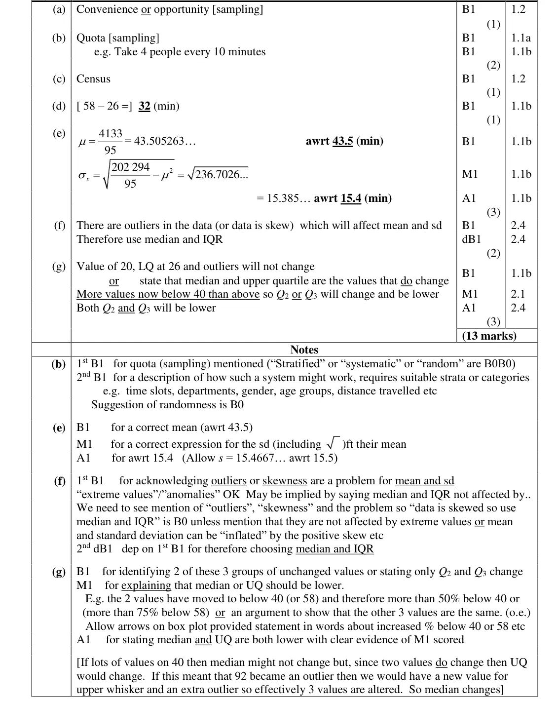
whole of section A. Part (f) was a familiar type of question from the legacy S1 specification but, although many identified the median and interquartile range as being the preferred statistics to use far fewer gave a reason to support this based on the presence of the outliers.
Common mistakes
outliers (or skew) affect mean and sd so use median and IQR
must give the reason, not just the choice
"skewed so use median" alone is B0
June 2018 · Paper 3 · Q4(g)3 marks
Mark scheme (whole question; this part is marked with the orange bar)
Examiner's comment
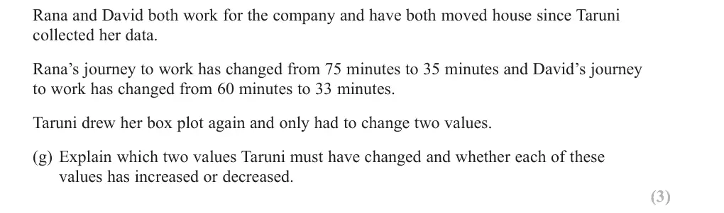
In part (g) most students identified that the median and upper quartile would change but few could give an adequate and accurate description to explain why. Many explained that the two values have moved to below 40 but failed to go on to explain that this would mean that there were more than 50% of the values below 40 and so the median of 40 would need to be lower. There were a number of students referring to changes in the mean and standard deviation despite these values not appearing in a box plot. It is hoped that over time students will get better at giving the level of detail in explanation that the new specification requires.
Common mistakes
minimum, LQ and outliers unchanged
two values move below 40 so more than 50% below 40 (and more than 75% below 58): median and UQ both decrease
mean and sd are not on a box plot
Find an Edexcel maths tutor
Stuck on this? Book a trial session with an Edexcel specialist.