Paper 2, Paper 2 (Statistics), Paper 3, Paper 3 (Statistics)
Level
AS and A level
Spec
S2.2
Booklet
Critical values for the product-moment correlation coefficient are given.
Since 2018
40 question parts, 59 marks
Notes, worked examples and practice for this topic are being written by our tutors. The past-paper questions below are ready now: work each one on paper, then open the mark scheme and the examiner's comment.
Tap a question to zoom it. Mark scheme and examiner's comment open under each question.
June 2025 · AS Paper 2 (Statistics) · Q4(b)(i)2 marks
Mark scheme (whole question; this part is marked with the orange bar)
Examiner's comment
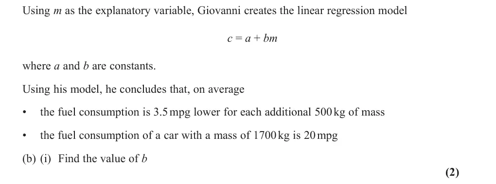
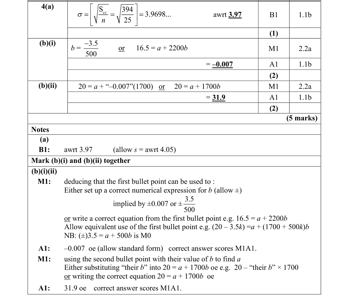
For part (b) many students misinterpreted the information in the first bullet point and used the incorrect equation 3.5 = a + 500b together with the correct one of 20 = a + 1700b. Those who had interpreted the information correctly generally used it in conjunction with the second bullet point to obtain 16.5 = a + 2200b as their equation together with 20 = a + 1700b ∓3.5 although a few of those using this approach used 1200b instead of 2200b. 500 were more successful although some of Those who used the gradient approach with b = these did not pick up that the gradient was negative. There were some students who had the gradient upside down.
Common mistakes
gradient b = −3.5/500 = −0.007 (negative, not upside down)
3.5 = a + 500b is wrong (common misreading of the first bullet)
alternatively 16.5 = a + 2200b with 20 = a + 1700b
June 2025 · AS Paper 2 (Statistics) · Q4(b)(ii)2 marks
Mark scheme (whole question; this part is marked with the orange bar)
Examiner's comment
In part (a), it appeared that many students did not recognise the sum given as that used in the Common errors were sqrt 394 and 394 original definition of variance/standard deviation and so were unable to attempt an answer. 25 although other wrong solutions involving extensive calculations were also seen. For part (b) many students misinterpreted the information in the first bullet point and used the incorrect equation 3.5 = a + 500b together with the correct one of 20 = a + 1700b. Those who had interpreted the information correctly generally used it in conjunction with the second bullet point to obtain 16.5 = a + 2200b as their equation together with 20 = a + 1700b ∓3.5 although a few of those using this approach used 1200b instead of 2200b. 500 were more successful although some of Those who used the gradient approach with b = these did not pick up that the gradient was negative. There were some students who had the gradient upside down.
Common mistakes
substitute their b into 20 = a + 1700b to get a = 31.9
1200b used instead of 2200b in the simultaneous-equation approach
June 2025 · Paper 3 (Statistics) · Q4(c)2 marks
Mark scheme (whole question; this part is marked with the orange bar)
Examiner's comment
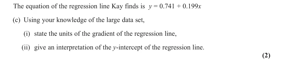
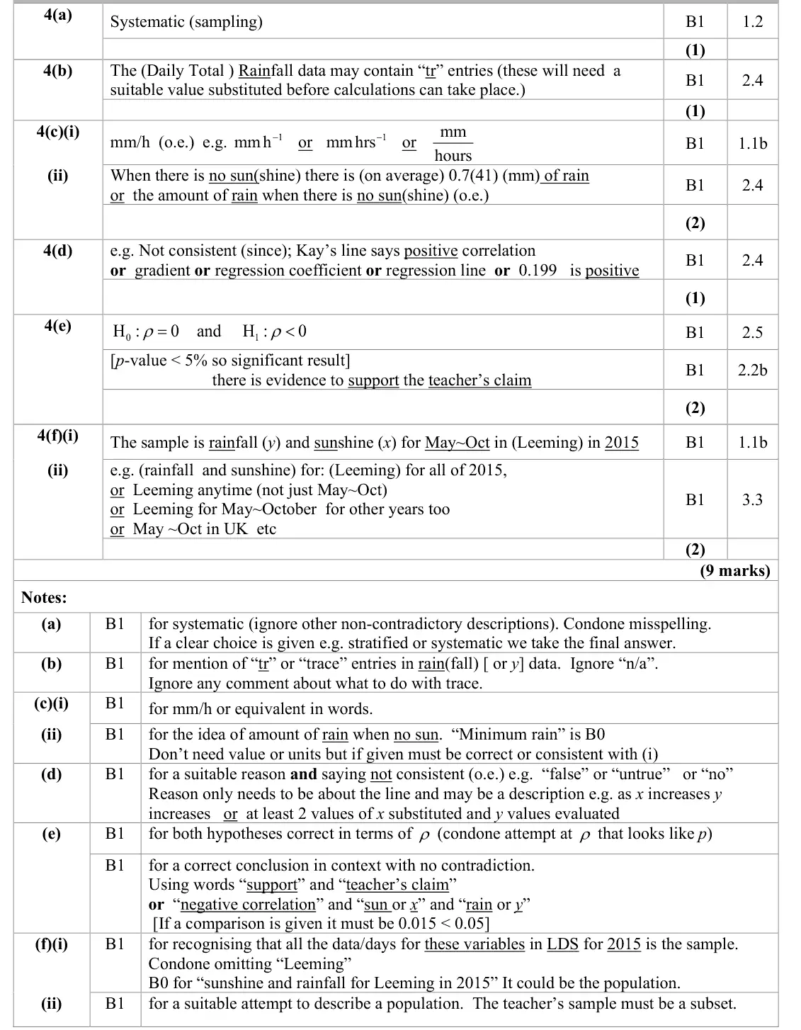
to the rainfall variable. In part (c) (i) there were many correct answers and some who identified mm or hours but not in a correct combination: answers such as mm2 or even -were seen, whilst others appeared not to be that familiar with the large data set and 1 hour mm used other incorrect units such as oktas, lumens or Hpa. Most responses gave a suitable contextual response to part (ii) but some simply said that 0.714 was the minimum rainfall rather than the (average) rainfall when there was no sun. The majority of responses recognised the inconsistency between Kay’s teacher’s claim and Kay’s data and many cited “positive correlation” for Kay’s data as their reason. A few opted to substitute two different values into the equation of the line to demonstrate their point. A small minority believed the teacher’s claim to be true and they were perhaps relying on their knowledge of weather conditions rather than interpreting the data Kay had collected.
Common mistakes
units of the gradient mm per hour (rainfall mm, sunshine hours), not oktas or hPa
intercept = (average) rainfall when there is no sunshine, not "minimum rainfall"
June 2025 · Paper 3 (Statistics) · Q4(d)1 mark
Mark scheme (whole question; this part is marked with the orange bar)
Examiner's comment
On the whole this question proved quite challenging as it tested a number of topics: sampling, regression, correlation and hypothesis testing as well as using the large data set and having a number of parts requiring a written explanation. However, there was something for all
Common mistakes
not consistent: Kay's gradient 0.199 is positive (positive correlation)
use the data, not weather knowledge
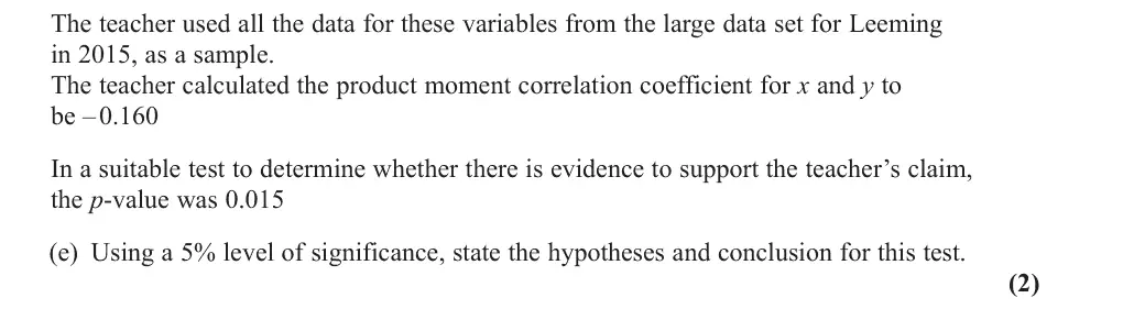
June 2025 · Paper 3 (Statistics) · Q4(e)2 marks
Mark scheme (whole question; this part is marked with the orange bar)
Examiner's comment
learners and very few blank responses were seen and parts (e) and (f) provided an opportunity for differentiation. Part (e) was found to be much more challenging for learners. Many were able to state the hypotheses correctly although some had an alternative hypothesis of ρ >0 and a few had a null hypothesis of ρ = 0.015 though few were using r instead of ρ. Very few responses interpreted the p-value with many comparing it to 0.16 or comparing 0.16 with 0.05 but some gave a correct conclusion in context. Good attempts to part (f) were rare and blank responses
Common mistakes
H₀: ρ = 0, H₁: ρ < 0 (not ρ > 0, not r, not 0.015)
compare the p-value 0.015 with 0.05 (not −0.160)
conclude in context: evidence to support the teacher's claim
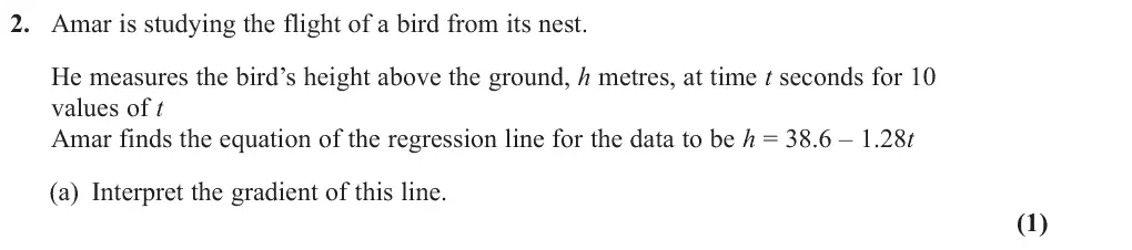
June 2024 · Paper 3 (Statistics) · Q2(a)1 mark
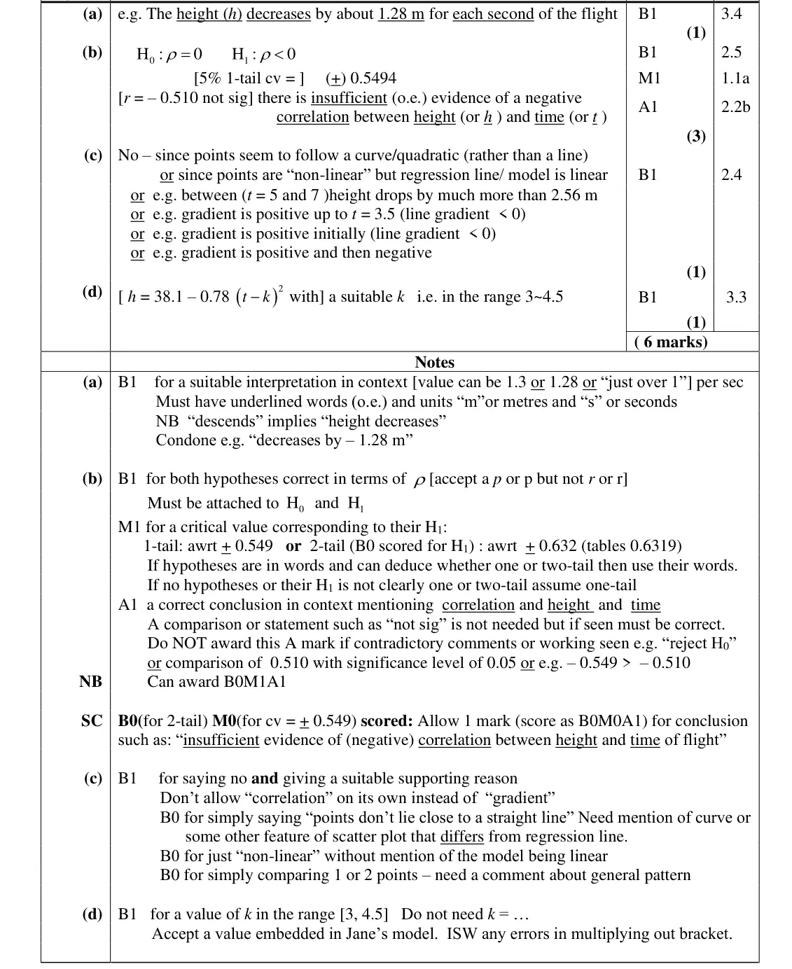
Mark scheme (whole question; this part is marked with the orange bar)
Examiner's comment
Whilst most students showed they had a good grasp of the concepts of correlation and regression some failed to give sufficient detail in their answers. In part (a) the requirement to “interpret” meant, as usual, that we needed a fully contextual response. Some simply stated “negative correlation” or gave the value of the gradient as – 1.28 whereas a full interpretation of the rate expected to see mention of the height decreasing by 1.28 m(etres) for each second of flight. In part (b) most students interpreted this situation as a one-tailed test and stated the
Common mistakes
height decreases by about 1.28 m for each second of flight (units and context needed)
"negative correlation" or just −1.28 not an interpretation
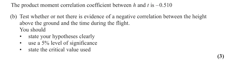
June 2024 · Paper 3 (Statistics) · Q2(b)3 marks
Mark scheme (whole question; this part is marked with the orange bar)
Examiner's comment
Whilst most students showed they had a good grasp of the concepts of correlation and flight. In part (b) most students interpreted this situation as a one-tailed test and stated the hypotheses correctly in terms of but a few equated this equal to – 0.510 rather than 0 for the null hypothesis. Almost all the students gave a critical value that matched their alternative hypothesis, and an encouraging number gave a correct contextual conclusion to the test mentioning both height and time. Some however lost the final accuracy mark for having contradictory or incorrect statements such as “reject H0” followed by a correct contextual conclusion such as “there is insufficient evidence of a negative correlation between h and t”. Although we did not require a comparison of the test statistic with the critical value if one was seen it had to be correct and some students lost the final mark for statements such as – 0.510 < – 0.5494 or for comparing 0.510 with the significance level of 0.05 In part (c) most
Common mistakes
H₀: ρ = 0, H₁: ρ < 0 (not ρ = −0.510, not r)
one-tail cv 0.5494
not significant: insufficient evidence of negative correlation between height and time
no contradictory "reject H₀"
do not compare r with 0.05
June 2024 · Paper 3 (Statistics) · Q2(c)1 mark
Mark scheme (whole question; this part is marked with the orange bar)
Examiner's comment
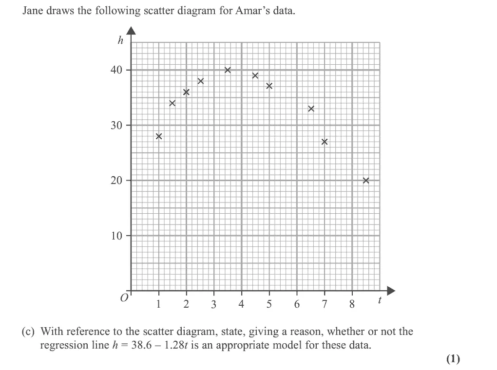
Whilst most students showed they had a good grasp of the concepts of correlation and – 0.510 < – 0.5494 or for comparing 0.510 with the significance level of 0.05 In part (c) most students realised that the given equation was not an appropriate model but did not give a strong enough explanation as to why this was so. Those who noted that the scatter diagram showed a curved set of data scored the mark whilst those who suggested that the points seemed to form a score the mark in part (c) some simply discussed correlation rather than stating that the line had negative gradient throughout whereas the scatter diagram had a positive gradient initially and then a negative gradient. Others just compared one or two points rather than concentrating on the overall shape of the scatter diagram and some simply stated “non-linear” without developing their answer and drawing out a difference between the scatter diagram and Amar’s linear model.
Common mistakes
not appropriate: points follow a curve (gradient positive then negative) but the line is linear
bare "non-linear", "not close to a line", correlation talk or comparing one or two points not enough
June 2024 · Paper 3 (Statistics) · Q2(d)1 mark
Mark scheme (whole question; this part is marked with the orange bar)
Examiner's comment
Whilst most students showed they had a good grasp of the concepts of correlation and (negative) quadratic probably also gave themselves lead in to part (d). Of those who did not score the mark in part (c) some simply discussed correlation rather than stating that the line had Part (d) proved challenging for most students and many simply moved on to the next question. There were many convoluted attempts involving calculus or multiplying out the bracket or substituting a value such as (1, 28). Students should be encouraged to consider the number of marks available as a guide to the amount of work required to answer the question. Those who had identified the scatter diagram as representing a parabola and saw the connection with the quadratic nature of Jane’s model could simply estimate the equation of the axis of symmetry and usually chose a suitable value of k.
Common mistakes
k is the t value of the vertex (axis of symmetry) of the curved scatter, any k in 3 to 4.5
1 mark so no calculus or expanding needed
June 2023 · AS Paper 2 (Statistics) · Q2(a)1 mark
Mark scheme (whole question; this part is marked with the orange bar)
Examiner's comment
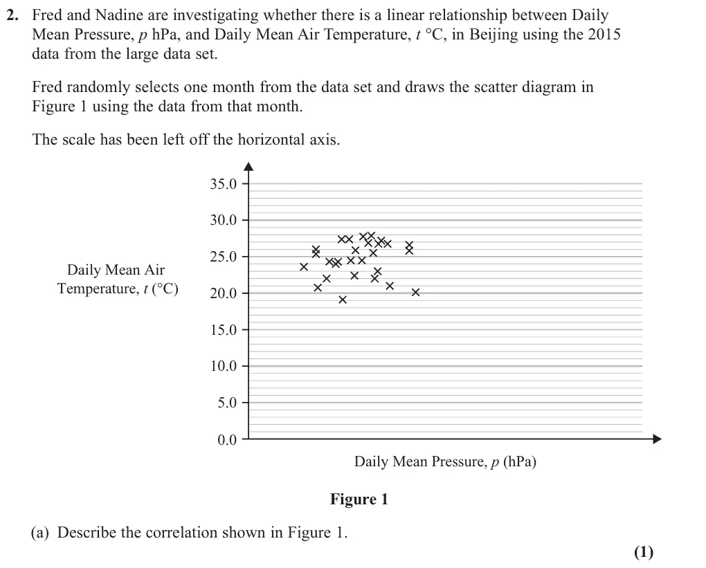
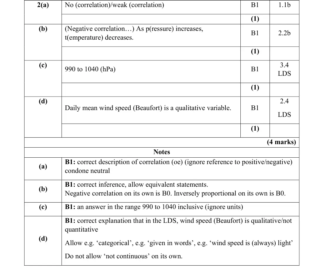
This question was the second most accessible question on the paper thanks to part (a) and (b), but due to parts (c) and (d) requiring familiarity with the large data set, only a small minority Most students successfully answered part (a) with a correct interpretation of a lack of correlation shown in Figure 1.
Common mistakes
no (or weak) correlation
positive/negative ignored
June 2023 · AS Paper 2 (Statistics) · Q2(b)1 mark
Mark scheme (whole question; this part is marked with the orange bar)
Examiner's comment
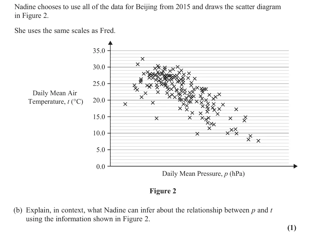
This question was the second most accessible question on the paper thanks to part (a) and (b), but due to parts (c) and (d) requiring familiarity with the large data set, only a small minority Part (b) was also answered well with students answering in the context of temperature and pressure. There were some students who did not earn the mark as they only wrote negative correlation and others that described a negative correlation as one quantity decreasing as the other decreased. It was notable that many students are still unfamiliar with the large data set and the general standard in parts (c) and (d) was poor. Most students guessed an answer to part (c) but very
Common mistakes
must interpret in context: as pressure increases temperature decreases
"negative correlation" alone or "inversely proportional" scores 0
June 2023 · AS Paper 2 (Statistics) · Q2(c)1 mark
Mark scheme (whole question; this part is marked with the orange bar)
Examiner's comment
but due to parts (c) and (d) requiring familiarity with the large data set, only a small minority of students scored full marks here. Most students successfully answered part (a) with a correct interpretation of a lack of standard in parts (c) and (d) was poor. Most students guessed an answer to part (c) but very few were able to give an answer in the correct range. In part (d), the students often described
Common mistakes
interpolation needs a pressure within the LDS range for Beijing 2015, 990 to 1040 hPa
most students guessed
June 2023 · AS Paper 2 (Statistics) · Q2(d)1 mark
Mark scheme (whole question; this part is marked with the orange bar)
Examiner's comment
but due to parts (c) and (d) requiring familiarity with the large data set, only a small minority of students scored full marks here. Most students successfully answered part (a) with a correct interpretation of a lack of standard in parts (c) and (d) was poor. Most students guessed an answer to part (c) but very few were able to give an answer in the correct range. In part (d), the students often described the location of Beijing as a factor or repeated an answer given in previous examination series rather than comment on the Beaufort Conversion being qualitative data. It was clear the students who had studied the large data set as their answers had a concise explanation.
Common mistakes
Daily Mean Wind Speed (Beaufort Conversion) is qualitative/categorical (given in words)
"not continuous" alone not accepted
location of Beijing is not a reason
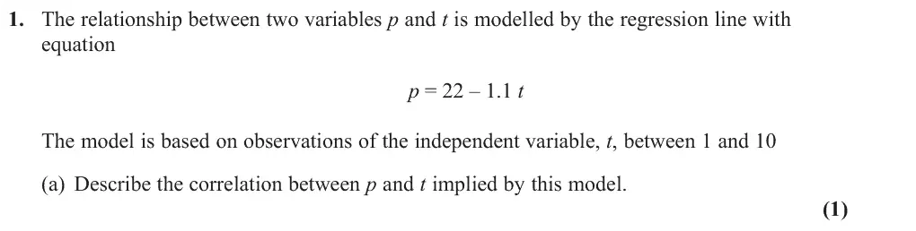
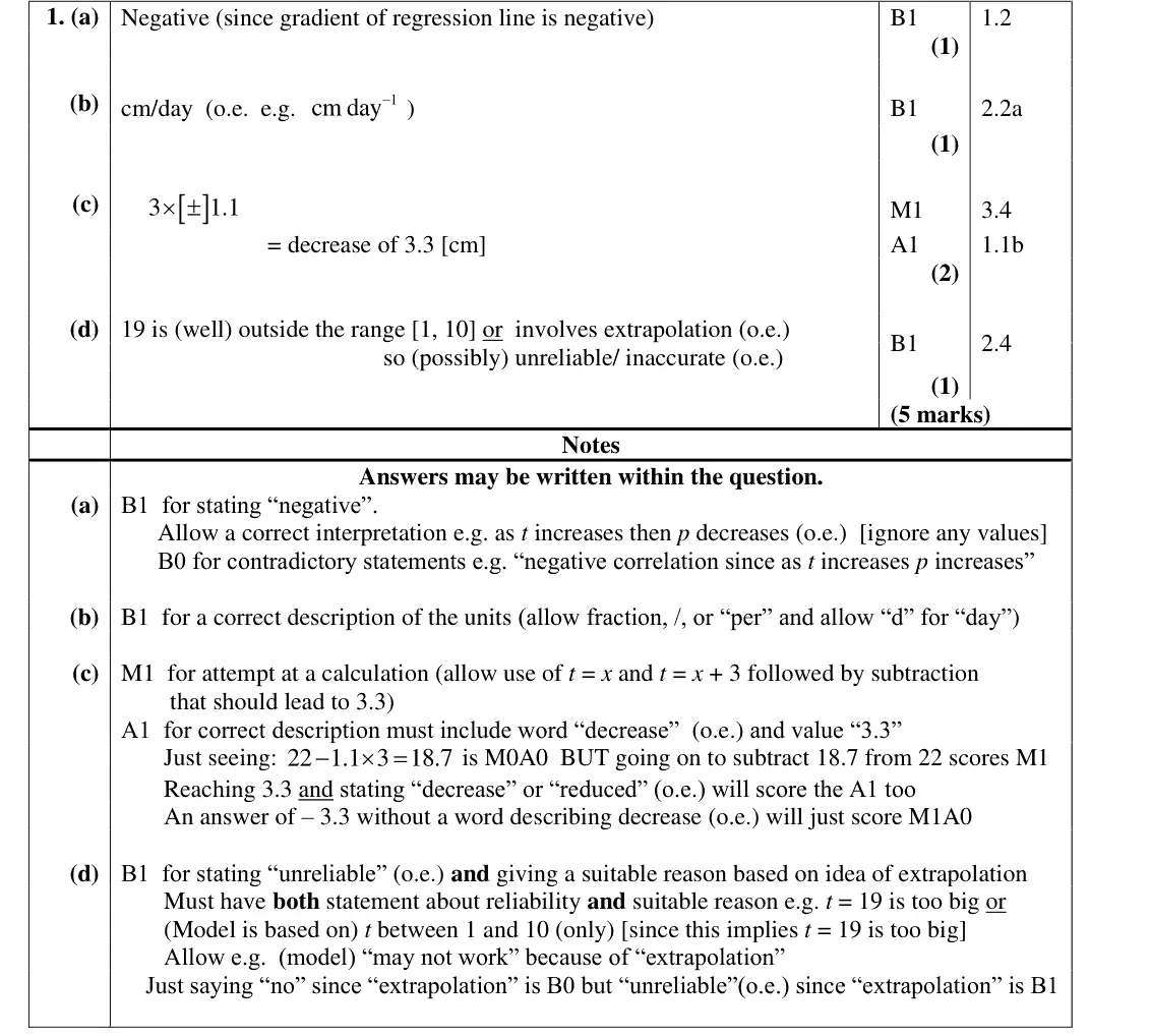
June 2022 · AS Paper 2 (Statistics) · Q1(a)1 mark
Mark scheme (whole question; this part is marked with the orange bar)
Examiner's comment
Part (a) was answered well with most stating that the correlation was negative or in a few cases giving us a suitable description such as “t increases as p decreases”. It was encouraging to see most giving a suitable description of the units for the gradient in part (b) too although some simply said
Common mistakes
"negative" (or as t increases p decreases)
contradictory statements score 0
June 2022 · AS Paper 2 (Statistics) · Q1(b)1 mark
Mark scheme (whole question; this part is marked with the orange bar)
Examiner's comment
giving a suitable description of the units for the gradient in part (b) too although some simply said “days” having failed to appreciate that the gradient represented a rate. In part (c) some simply
Common mistakes
gradient is a rate: cm per day (cm/day)
"days" alone scores 0
June 2022 · AS Paper 2 (Statistics) · Q1(c)2 marks
Mark scheme (whole question; this part is marked with the orange bar)
Examiner's comment
“days” having failed to appreciate that the gradient represented a rate. In part (c) some simply substituted t = 3 into the equation and gained no marks but most used t = 3 and t = 0 and subtracted to obtain a value of + 3.3 A sizeable minority thought that using t = 3 and t = 1 would give them the change over 3 days. Few though told us though that this change represented a decrease in p and so that last mark was rarely scored. The responses to part (d) were encouraging. Most secured the
Common mistakes
3 × 1.1 = 3.3
must say "decrease" (−3.3 alone is M1A0, rarely given full marks)
substituting t = 3 alone scores 0
t = 3 and t = 1 is not a 3-day change
June 2022 · AS Paper 2 (Statistics) · Q1(d)1 mark
Mark scheme (whole question; this part is marked with the orange bar)
Examiner's comment
that last mark was rarely scored. The responses to part (d) were encouraging. Most secured the mark by stating that the estimate would be unreliable and either mentioned that the data were bases on values of t between 1 and 10 or said that using 19 involved extrapolation. A common incorrect answer argued that because the estimate was still positive when t = 19 the estimate was reliable.
Common mistakes
unreliable because t = 19 is outside 1 to 10 (extrapolation)
both a judgement and a reason needed
"positive estimate so reliable" is wrong
June 2022 · Paper 3 (Statistics) · Q6(a)1 mark
Mark scheme (whole question; this part is marked with the orange bar)
Examiner's comment
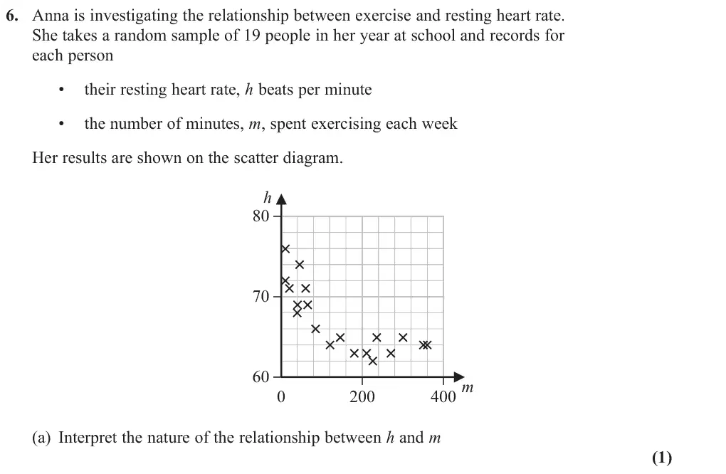
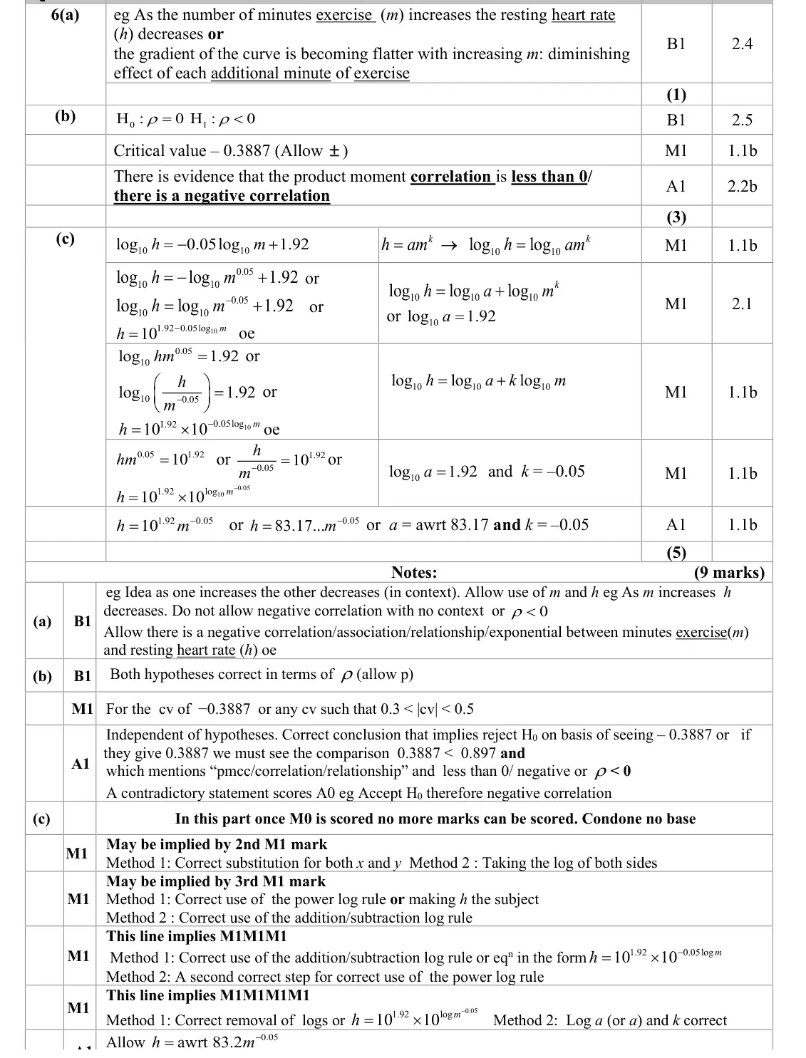
In part (a) a large number of students simply wrote ‘negative correlation’, with no context. The word Interpret in the question hints that context is required. Of the students that did try to truly interpret the correlation in a contextual statement, the vast majority were successful. Whilst many students realised that one- tailed hypotheses were needed in part (b) few
Common mistakes
in context: as minutes of exercise increase, resting heart rate decreases (with diminishing effect)
"negative correlation" with no context scores 0
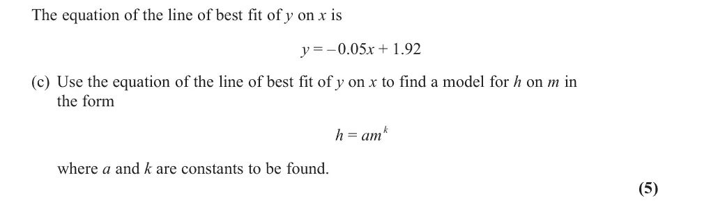
June 2022 · Paper 3 (Statistics) · Q6(c)5 marks
Mark scheme (whole question; this part is marked with the orange bar)
Examiner's comment
In part (a) a large number of students simply wrote ‘negative correlation’, with no context. The word Interpret in the question hints that context is required. Of the students that did try to truly interpret the correlation in a contextual statement, the vast majority were successful. Whilst many students realised that one- tailed hypotheses were needed in part (b) few used ρ for the parameter. Most students had ± the correct CV but the final A1 was lost by many students, as they compared the positive value 0.3887 to the negative test statistic. This showed these students were unfamiliar with the meaning of the CV/CR and how it related to their test statistic. Part (d) differentiated well between students with basic knowledge and those with deeper understanding. The majority of students scored 5/5 on this part. Almost all used the LH approach on the MS. This was usually well done, though a good number made errors with the laws of indices and maintained a + between the two terms after making the equation into powers of 10. The students knew their log rules, but many did only so to a basic degree, and came unstuck during their working. Sometimes this was to such an extent that they lost the marks. A surprisingly high number of students used natural logarithms and hence the exponential function in this question showing a less secure grip of this topic.
Common mistakes
substitute x = log₁₀m, y = log₁₀h
power and addition log laws
h = 10^1.92 × m^−0.05 = 83.2m^−0.05
keep the plus inside the log, not between powers of 10
use log base 10, not ln
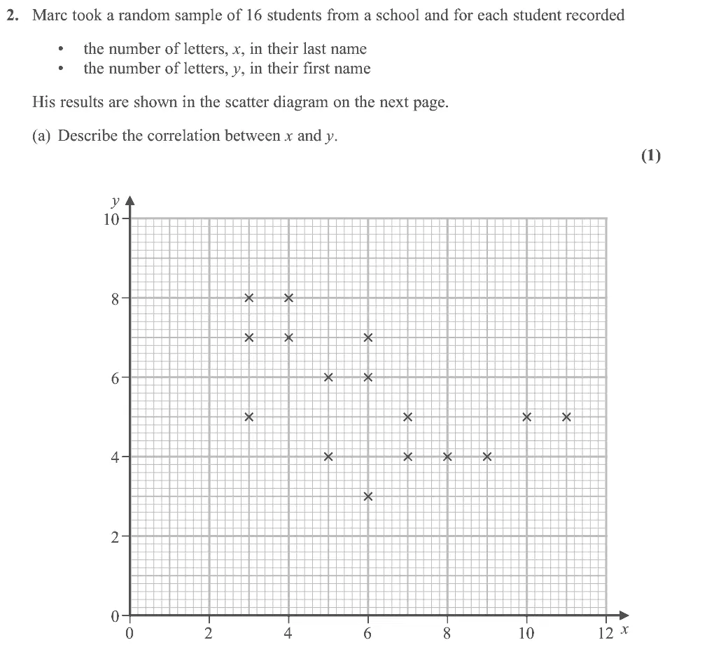
Oct 2021 · Paper 3 (Statistics) · Q2(a)1 mark
Mark scheme (whole question; this part is marked with the orange bar)
Examiner's comment
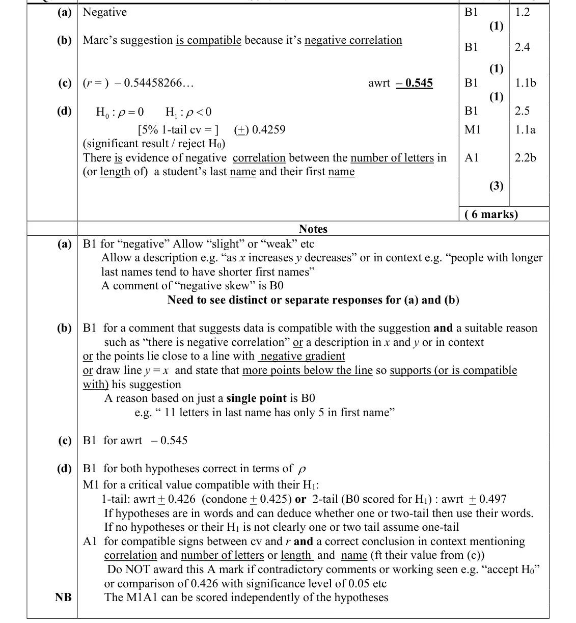
Most scored the mark in part (a) by identifying that the correlation was negative. When we ask students to “describe” we are simply requiring a non-contextual description. We will ask them to “interpret” when we require a contextual description. In this case we allowed students to describe the correlation in terms of the variables so answers such as “as x increases y decreases” were accepted. Some thought the correlation was strong and others weak but at this stage all we wanted was the negative description. Part (b) caused some
Common mistakes
"negative" (strength not needed)
"negative skew" is B0
describe needs no context
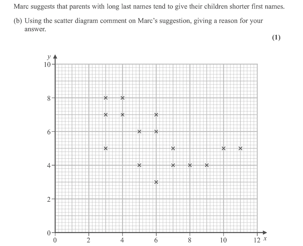
Oct 2021 · Paper 3 (Statistics) · Q2(b)1 mark
Mark scheme (whole question; this part is marked with the orange bar)
Examiner's comment
strong and others weak but at this stage all we wanted was the negative description. Part (b) caused some problems with some stating that the scatter diagram showed negative correlation but failing to say whether or not this was compatible with Marc’s suggestion. Some students felt that there was no correlation shown by the scatter diagram and did not reconsider this even after correctly answering part (d).
Common mistakes
must say the data are compatible with/support the suggestion AND give the reason (negative correlation)
a reason based on a single point scores B0
Oct 2021 · Paper 3 (Statistics) · Q2(c)1 mark
Mark scheme (whole question; this part is marked with the orange bar)
Examiner's comment
Most answered part (c) correctly though a number “lost” the minus sign between their calculator and writing down the answer on the page. Usually there were sufficient figures given for us to award the mark when the minus sign was included. In part (d) most attempted the hypotheses and the majority used ρ. Some
Common mistakes
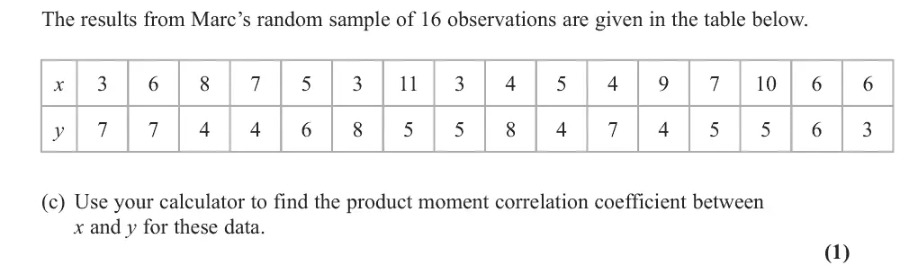
calculator r = −0.545
do not lose the minus sign
Oct 2020 · AS Paper 2 (Statistics) · Q2(b)2 marks
Mark scheme (whole question; this part is marked with the orange bar)
Examiner's comment
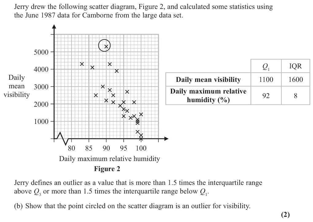
It was clear from the responses seen here that many candidates have little or no In part (b) most candidates who produced an answer were able to gain some marks. The most common mistake was to multiply the LQ by 3 in order to find the UQ. A few candidates calculated the upper boundary correctly, but then failed to make a comparison to finish off their reasoning.
Mark scheme (whole question; this part is marked with the orange bar)
Examiner's comment
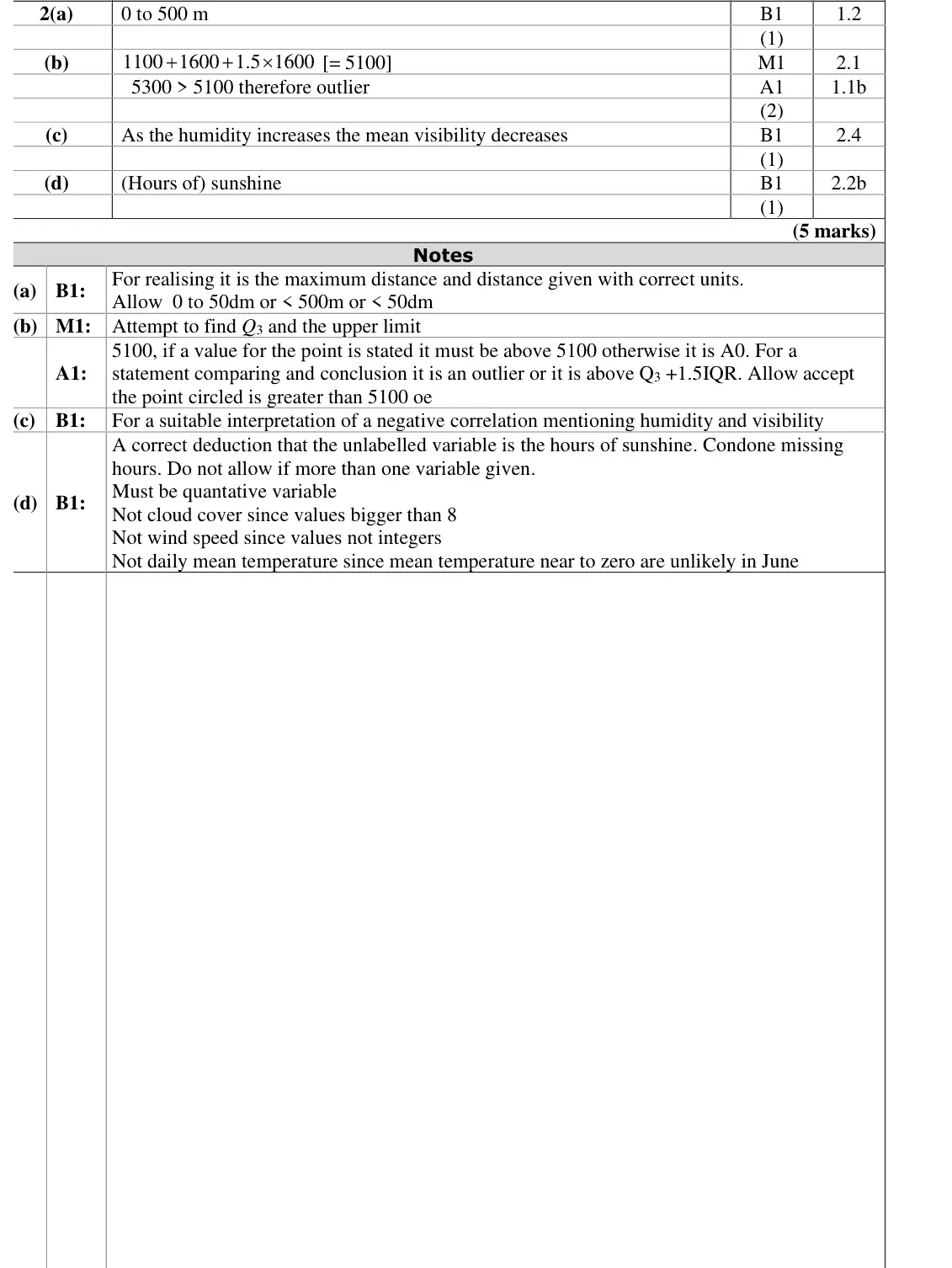
It was clear from the responses seen here that many candidates have little or no In part (c) too many candidates simply wrote negative correlation. The demand interpret the correlation requires an explanation in context of what this means.
Common mistakes
negative correlation must be interpreted in context (as humidity increases visibility decreases)
just "negative correlation" scores 0
Oct 2020 · AS Paper 2 (Statistics) · Q2(d)1 mark
Mark scheme (whole question; this part is marked with the orange bar)
Examiner's comment
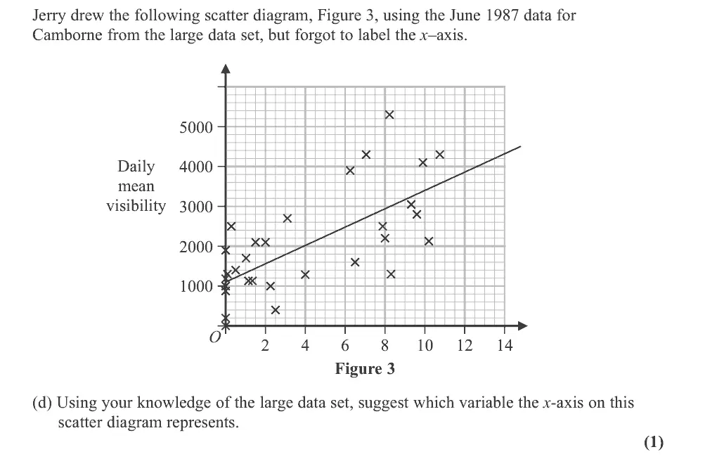
It was clear from the responses seen here that many candidates have little or no figures for Daily Mean Visibility are in decametres (Dm). In part (d) a minority of students gave the correct variable hours of sunshine (just Sunshine was accepted) as the variable.
Common mistakes
(hours of) sunshine
not cloud cover (values above 8 oktas), not wind speed (values not integers), not mean temperature (near-zero unlikely in June)
give one variable only
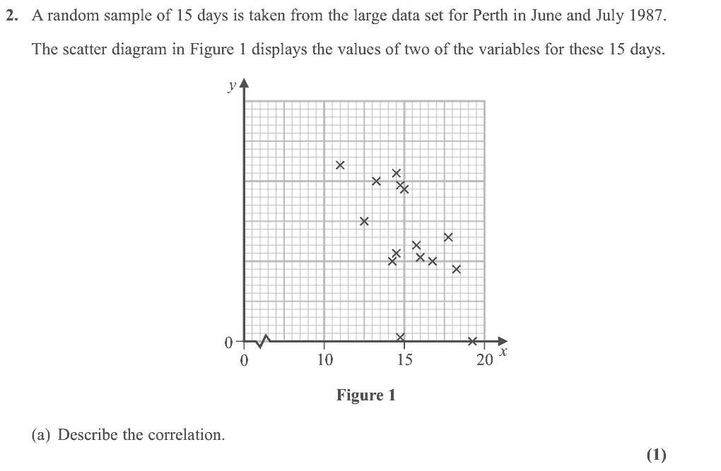
Oct 2020 · Paper 3 (Statistics) · Q2(a)1 mark
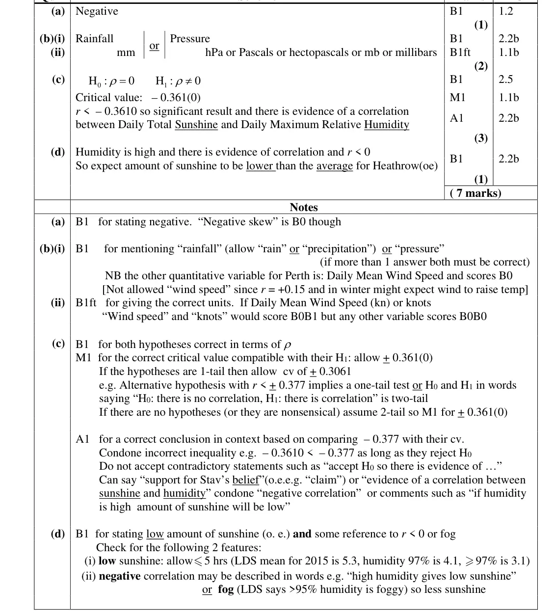
Mark scheme (whole question; this part is marked with the orange bar)
Examiner's comment
Very few students were unable to identify the negative correlation in part (a) with many attempting to describe the strength as well (split fairly evenly between weak and strong) though this was not required here. In part (b) it was clear that more students were
Common mistakes
negative (strength not required)
"negative skew" is wrong
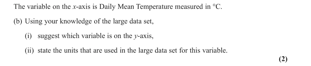
Oct 2020 · Paper 3 (Statistics) · Q2(b)2 marks
Mark scheme (whole question; this part is marked with the orange bar)
Examiner's comment
though this was not required here. In part (b) it was clear that more students were familiar with the large data set. Many identified “rainfall” as the variable on the y-axis and they usually gave the correct units although some thought it should be mm3. The most common incorrect answer here was “cloud cover” but, of course, this variable is not available on the large data set for Perth. Part (c) was a standard hypothesis test for
Common mistakes
Perth has no cloud cover
rainfall (mm) or pressure (hPa) – the only other Perth variable, wind speed, is positively correlated with temperature
mm³ is wrong
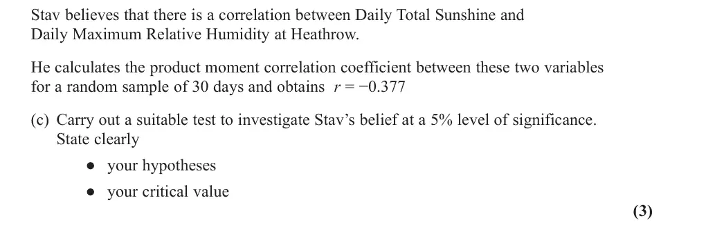
Oct 2020 · Paper 3 (Statistics) · Q2(c)3 marks
Mark scheme (whole question; this part is marked with the orange bar)
Examiner's comment
not available on the large data set for Perth. Part (c) was a standard hypothesis test for correlation. It was encouraging to see a good number using ρ for the hypotheses but fewer realised that the test was two-tailed. The phrase “…believes there is a correlation between…” shows that a two tailed test should be used, however many were swayed by the negative value of r and opted for a one tailed test. It was good to see that most chose the critical value from the tables that was compatible with their alternative hypothesis and this meant that they could also access the final mark provided their comment was in context, “support for Stav’s belief” was perhaps the simplest way of including the context. There were some good answers to part (d) but many others were
Common mistakes
"a correlation" means a two-tailed test: H₀: ρ = 0, H₁: ρ ≠ 0 (many chose one tail because r < 0)
critical value −0.3610
conclusion in context (support for Stav's belief)
Oct 2020 · Paper 3 (Statistics) · Q2(d)1 mark
Mark scheme (whole question; this part is marked with the orange bar)
Examiner's comment
including the context. There were some good answers to part (d) but many others were unable to pull together the various parts of the question to make a correct inference. Some stated that the humidity was high and other assumed this but interpreted the negative value of r correctly and were then able to state that they would expect the number of hours of sunshine to be low. Some gave a suggested value for the number of hours of sunshine but this needed to be realistic and values more than 5 were not accepted. A few students knew (from the large data set) that humidity greater than 95% implies foggy conditions and argued correctly that this would suggest a low amount of sunshine.
Common mistakes
high humidity with negative correlation (or fog above 95% humidity) means low sunshine, below the Heathrow average
a suggested value must be realistic (5 hours or less)
June 2019 · AS Paper 2 (Statistics) · Q1(b)1 mark
Mark scheme (whole question; this part is marked with the orange bar)
Examiner's comment
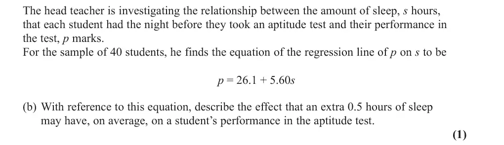
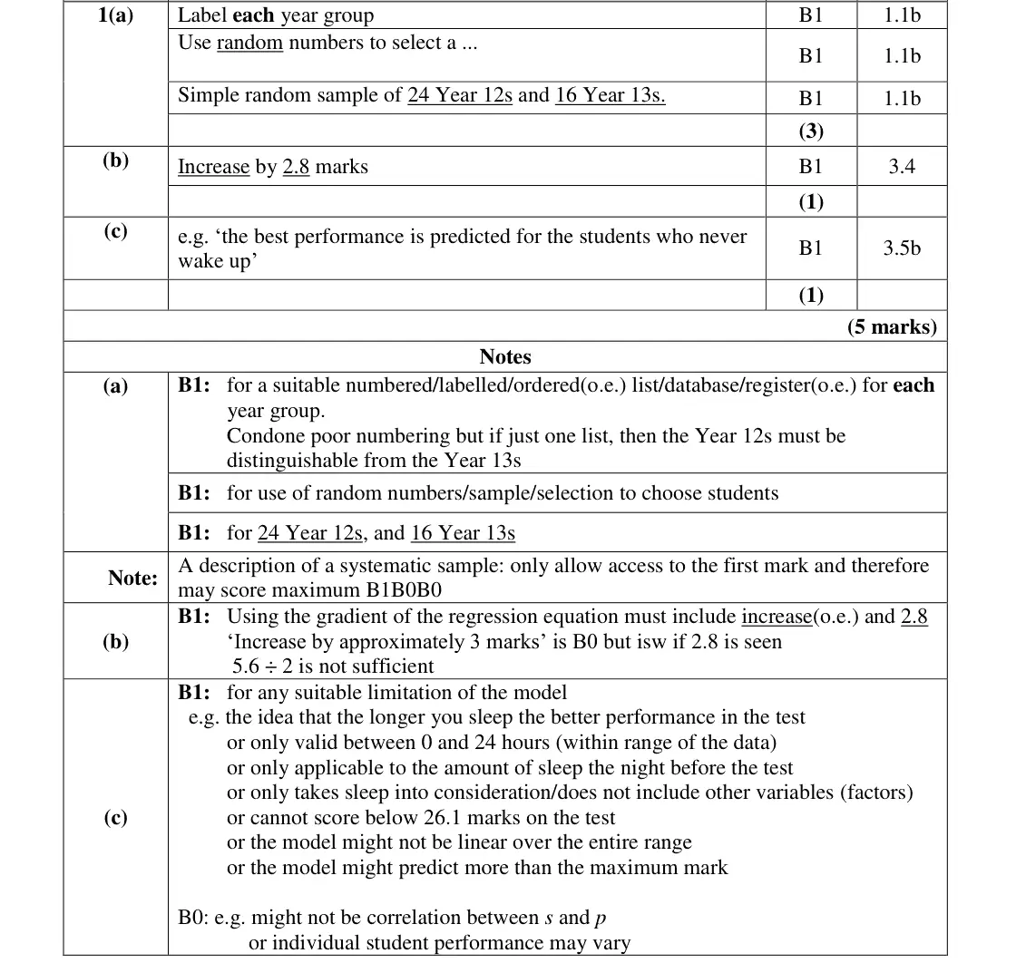
In part (b), most candidates scored the mark for indicating both ‘increase’ and ‘2.8’. A minority however worked out the number of points scored when s = 0.5. Others just mentioned the ‘increase’ but failed to quantify it appropriately.
Common mistakes
use the gradient: 0.5 × 5.60 = increase of 2.8 marks (both "increase" and 2.8 needed)
not the value of p at s = 0.5
"about 3 marks" is B0
June 2019 · AS Paper 2 (Statistics) · Q1(c)1 mark
Mark scheme (whole question; this part is marked with the orange bar)
Examiner's comment
Part (c) was very well answered and most gained a mark here by coming up with a plausible limitation of the model. The majority referred to ‘other factors affecting performance’ or ‘not specifying a range so candidates could not score less than 26.1 marks or could get infinitely high marks’.
Common mistakes
e.g. predicts best performance for students who never wake up, only valid within the range of the data, ignores other factors, could exceed the maximum mark
"might not be correlation" is not accepted
June 2019 · Paper 3 (Statistics) · Q3(b)1 mark
Mark scheme (whole question; this part is marked with the orange bar)
Examiner's comment
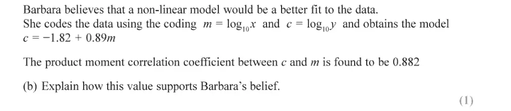
This was the second most successful question on the paper with nearly a quarter of candidates Many gave a correct response in part (b) using the idea that the correlation was stronger or the value closer to 1. Some candidates only compared the value of 0.822 to 0.446 (or 0 or 0.3438) without explaining how this supported Barbara’s belief by showing a stronger correlation compared to the uncoded data. A common incorrect answer was to state that 0.882 was close to 0.89, the gradient of the regression equation. A variety of approaches were taken to answer part (c). Those that opted to take method 2
Common mistakes
0.882 is closer to 1 than 0.446 – stronger correlation for the log-coded data
just comparing with 0.3438 or saying 0.882 is close to the gradient 0.89 scores nothing
"association" not allowed
June 2019 · Paper 3 (Statistics) · Q3(c)5 marks
Mark scheme (whole question; this part is marked with the orange bar)
Examiner's comment
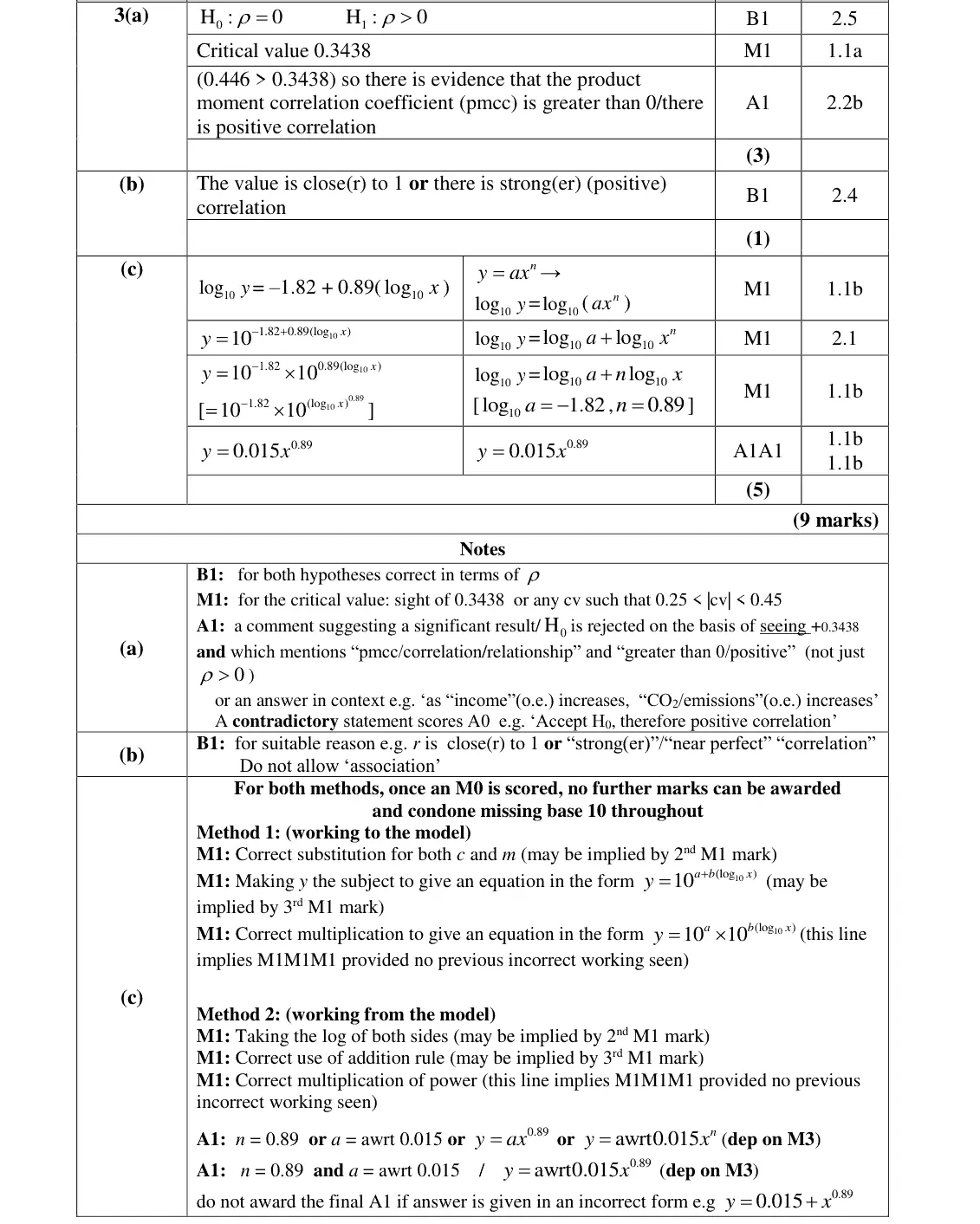
This was the second most successful question on the paper with nearly a quarter of candidates A variety of approaches were taken to answer part (c). Those that opted to take method 2 (working from the model) on the whole were usually more successful, as many could jump . A common error was to give n = 7.762… .0.89 log log log y a n x straight to 10 10 10 10 Those candidates that struggled with this question were able to score the first mark as many log 1.82 0.89(log ) y x could state but then failed to make y the subject. Even those 10 10 candidates that could deal with logarithms often lost the final mark as did not evaluate their 10 1.82 value of a (too many left this as ).
Common mistakes
log y = −1.82 + 0.89 log x
make y the subject: y = 10^−1.82 × x^0.89 = 0.015x^0.89
evaluate a (not left as 10^−1.82)
n = 0.89 not 10^0.89
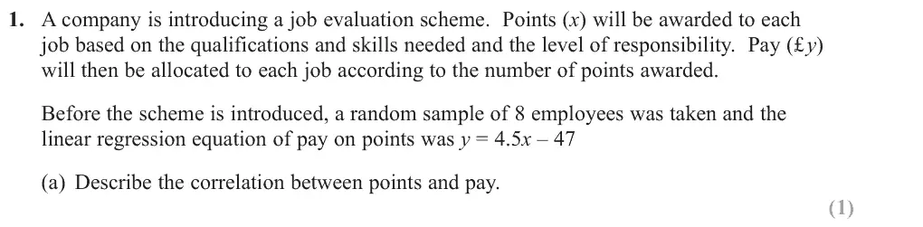
June 2018 · AS Paper 2 · Q1(a)1 mark
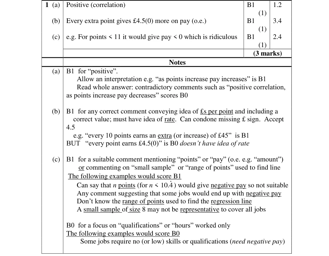
Mark scheme (whole question; this part is marked with the orange bar)
Examiner's comment
Part (a) proved an accessible starter for students with most students describing the correlation as positive as required. We use the command “interpret” when we expect a comment related to the context and “describe” when all we are looking for is a description of the statistic. In part (b), some
Common mistakes
positive (correlation)
"as points increase pay increases" is accepted
contradictory comments such as "positive, as points increase pay decreases" score 0
June 2018 · AS Paper 2 · Q1(b)1 mark
Mark scheme (whole question; this part is marked with the orange bar)
Examiner's comment
context and “describe” when all we are looking for is a description of the statistic. In part (b), some mention of the context and the idea of “rate” was required and we would also expect to see a mention of the correct value for the gradient. A typical answer was “an increase of 1 point gives an increase of £4.50 in pay”. In part (c), the students needed to engage with the model and explain why it might not
Common mistakes
each extra point gives £4.50 more pay: must convey a rate (£ per point) with the correct value and context
"every point earns £4.50" has no idea of rate
June 2018 · AS Paper 2 · Q1(c)1 mark
Mark scheme (whole question; this part is marked with the orange bar)
Examiner's comment
£4.50 in pay”. In part (c), the students needed to engage with the model and explain why it might not be suitable. One such reason focussed on the fact that for a score of less than 11 points the pay was negative which would not be reasonable. Some honed in on the small sample size and gave the sensible suggestion that the sample may not be large enough to be representative of all jobs in the company.
Common mistakes
fewer than about 10.4 points gives negative pay
a sample of 8 may not be representative of all jobs
the range of points used to find the line is unknown
comments only about qualifications or hours score 0
June 2018 · Paper 3 · Q2(b)1 mark
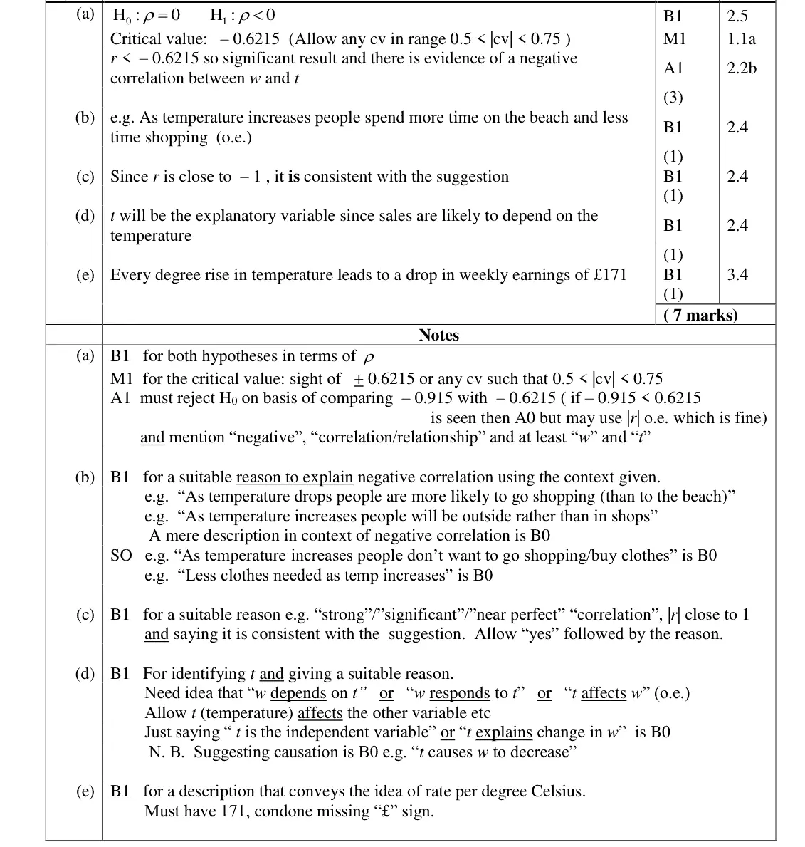
Mark scheme (whole question; this part is marked with the orange bar)
Examiner's comment
In part (b) some students identified that as the temperature increased more people would be outside visiting the beach perhaps rather than going shopping. There were several other less convincing suggestions made and some that would have suggested a positive correlation between weekly sales and temperature. Part (c) was answered very well, but in part (d) some students seemed unfamiliar
Common mistakes
must explain the negative correlation in context (e.g. hot weather, people at the beach rather than shopping)
a mere description of negative correlation is B0
June 2018 · Paper 3 · Q2(c)1 mark
Mark scheme (whole question; this part is marked with the orange bar)
Examiner's comment
and temperature. Part (c) was answered very well, but in part (d) some students seemed unfamiliar with the term, all that was required was the identification of temperature as the required variable and an explanation that, in this model, sales depend on or are affected by temperature. Part (e) was
Common mistakes
r close to −1 (strong/near perfect linear correlation) so consistent with a linear model
June 2018 · Paper 3 · Q2(d)1 mark
Mark scheme (whole question; this part is marked with the orange bar)
Examiner's comment
and temperature. Part (c) was answered very well, but in part (d) some students seemed unfamiliar with the term, all that was required was the identification of temperature as the required variable and an explanation that, in this model, sales depend on or are affected by temperature. Part (e) was
Common mistakes
t is explanatory because sales depend on temperature
"t is the independent variable" alone or suggesting causation is B0
June 2018 · Paper 3 · Q2(e)1 mark
Mark scheme (whole question; this part is marked with the orange bar)
Examiner's comment
an explanation that, in this model, sales depend on or are affected by temperature. Part (e) was answered well again with most mentioning the idea of rate and the relevant values.
Common mistakes
rate of change: each 1 °C rise in temperature, weekly sales fall by £171
must include 171
Find an Edexcel maths tutor
Stuck on this? Book a trial session with an Edexcel specialist.